A LOCAL SEQUENCE ALIGNMENT ALGORITHM USING AN ASSOCIATIVE MODEL OF PARALLEL COMPUTATION Shannon I. Steinfadt Department of Computer Science Kent State University Kent, Ohio 44242 USA
[email protected]
Michael Scherger Department of Computer Science Texas A & M University–Corpus Christi Corpus Christi Texas 78412 USA
[email protected]
ABSTRACT Local sequence alignment is widely used to discover structural and hence, functional similarities between biological sequences. While the faster heuristic methods like BLAST and FASTA are useful to compare a single sequence to hundreds or even thousands of sequences in genetic databases such as GenBank, EMBL, and DDBJ, this work yields pairwise alignments with a high sensitivity. The heuristic methods are ideal for narrowing down the number of “good” sequences. Rigorous alignment can then be utilized for an in-depth comparison between the query sequence and the newly found sequence subset. A data-parallel algorithm for local sequence alignment based on the Smith-Waterman algorithm has been adapted for an associative model of parallel computation known as ASC. The algorithm finds the best local alignment in O(m + n) time using m + 1 processing elements. KEY WORDS Computational techniques, sequence alignment, SmithWaterman algorithm, parallel computation, SIMD, associative computing
Johnnie W. Baker Department of Computer Science Kent State University Kent, Ohio 44242 USA
[email protected]
Approximate algorithms including BLAST [4], Gapped BLAST [5], and FASTA [6] are widely used due to their speed. Empirically, BLAST is 10-50 times faster than the Smith-Waterman algorithm [7]. The approximate algorithms were designed for speed, trading-off accuracy and sensitivity. Higher scoring subsequences can be missed due to the nature of the approximations. The heuristic algorithms are useful to help screen hundreds or thousands sequences to a reasonable set that can be studied more carefully with rigorous local alignment. As a result, a parallel exact sequence alignment with a reasonably large speedup over its sequential counterparts is desirable. This paper presents a local sequence alignment algorithm based on [3] using an associative model of computation known as ASC [8]. While other parallel versions of local sequence alignment algorithms exist for many different models of computation including SIMD [9][10][11] and MIMD [12] systems, this work extends local sequence alignment to the ASC model and serves as the foundation for finding the top k local alignments similar to SIM [13] and LALIGN [14] in the FASTA package [15] but with a much faster running time.
1. Introduction The alignment of two DNA or protein sequences is used to detect functional similarities. High sequence similarity implies structural and hence, functional similarity. The dynamic programming algorithms from Needleman and Wunsch [1] and Smith and Waterman [2] are exact alignment algorithms that find the highest scoring alignment possible between two DNA or protein strings. The Smith-Waterman algorithm with Gotoh optimizations [3] produces a local alignment with time and memory requirements proportional to the product of the two sequences’ length, or O(m •n). This quickly becomes computationally prohibitive as the size of the strings increase.
Section 2 outlines the Smith-Waterman algorithm, Section 3 introduces and explains the associative computing (ASC) model, and Section 4 discusses the associative local sequence alignment algorithm. The associative algorithm is compared to other similar algorithms in Section 5. Future work and the conclusions are covered in Sections 6 and 7. 2. The Smith-Waterman Algorithm Smith-Waterman is perhaps the most widely used local sequence alignment algorithm [16]. The dynamic programming method aligns the residues of two sequences S1 and S2. Gaps may be introduced into the original sequences during alignment. The goal is to maximize the
j
The Smith-Waterman algorithm is rigorous, checking every possible alignment via an m • n scoring matrix, where m is the length of S1 and n is the length of S2. A matrix element at location i,j in the matrix represents the score of an alignment ending at residue i of S1 and residue j of S2, where 0 ≤ i ≤ m and 0 ≤ j ≤ n. Scores in the first row and column are defined to be zero. The rest of the matrix is defined using the following recurrence relationships from [3]:
Pi. j Qi, j Di, j = MAX Di−1, j−1 + d ( S1i ,S2 j ) 0
1
Δ
G
P(0,0)=0
P(0,1)=0 Q(0,1)=0 D(0,1)=0
0 Δ Q(0,0)=0 D(0,0)=0
2 C
S2
P(0,2)=0 Q(0,2)=0 D(0,2)=0 2
P(1,0)=0
1 G Q(1,0)=0 D(1,0)=0
3
3
i P(2,0)=0 2 C Q(2,0)=0 D(2,0)=0
4
P(3,0)=0
3 C Q(3,0)=0 D(3,0)=0
(1) S1
€
Di−1, j + w1 Pi. j = MAX Pi−1, j + u
(2)
(3)
€
Di, j−1 + w1 Qi, j = MAX Qi, j−1 + u
€
0
diagonal
substring alignment of similar residues, indicating evolution similarity and lineage.
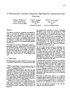
Di,j is the score of the best alignment ending at the position S1i, S2j, with the scoring function for a match or mismatch of the two residues d(S1i, S2j). Pi,j and Qi,j keep track of an insertion or deletion respectively, ending at S1i and S2j. The cost of introducing a single gap is represented by w 1 and u is the penalty of extending a gap by one. As shown in Equations 1-3, the score for each matrix element relies upon the previously computed scores for every element above (north of) it, to the left (west) of it, and on the diagonal (northwest) of it. This data dependency for one matrix element can be seen in Figure 1. The lightly shaded matrix element in the bottom right corner depends upon the three pre-computed matrix cells pointed to by the arrows. In turn, those three matrix cells rely on their own north, west, and northwest neighbors’ computations. By examining the data dependencies, the matrix elements along the anti-diagonals (shown by the dashed lines in Figure 1) do not require data from any other element along the anti-diagonal during their calculation. The values for these matrix elements and can be computed independently and in parallel using a wavefront method. The independence of matrix element computations along the anti-diagonal is exploited by the parallel algorithm presented in Section 4.
Figure 1. Sequential S-W matrix. The dark gray border blocks are initialized to zeros. The antidiagonals are shown as dashed lines. The lighter gray box at (i,j)=(3,2) shows the three values its data is dependent upon: northwest (i-1,j-1), north (i1,j) and west (i, j-1) or (2,1), (2,2) and (3,1).
Once the scoring matrix has been calculated for the sequential local alignment, the second phase of the algorithm identifies the best local alignments. Sequentially, the first part of the algorithm takes O(m • n) time, and the second part of the algorithm, known as traceback, can take up to O(m + n) time. Traceback is a dynamic process, and it depends upon the best alignment computed in the scoring matrix. Since the first phase is computationally intensive, it is the focus of the parallelization for the ASC model in this paper. 3. Associative Computing and the ASC Model of Parallel Computation A parallel associative model of computation [8] known as ASC (ASsociative Computing) is a generalized version of the associative computing style that has been in use since the 1970’s with the introduction of associative SIMD computers such as the STARAN. Associative computing includes the use of data parallel programming [17]. Unlike MIMD programming, ASC programmers are not responsible for load balancing, synchronization points, task allocation, scheduling, etc. Additionally, data is either broadcast or moved synchronously using the interconnection network thereby avoiding difficulties involving both message passing and shared memory. An ASC computer can handle real-time applications, such as collision avoidance in air traffic control (ATC) in low-order polynomial time [18][19]. The ASC model does not employ associative memory. The reference to the word “associative” is related to the use of searching to locate data by content rather than memory
address. The data remains in place in the responding processing elements (PEs) and these PEs are subsequently processed in parallel.
PE
Memory
PE
Memory
PE
Memory
PE
Memory
PE
Memory
PE
Memory
Cell / PE Interconnection Network
Instruction Stream
Broadcast / Reduction Network
As shown in Figure 2, the ASC model consists of an array of cells and a single instruction stream (IS). Each cell is composed of a PE and a local memory. Each PE is capable of performing local arithmetic, logical operations, and the usual functions of a sequential processor other than issuing instructions. Every PE listens to the IS, which broadcasts data and instructions. The term cell and PE are used interchangeably in this paper to refer to both the processing element and its local memory.
Figure 2: Conceptual view of the ASC model of parallel computation.
PEs in the ASC model can be active, inactive, or idle. The IS can broadcast to all of its cells but only the active PEs execute an associative search. Since only active PEs execute the instructions broadcast from the IS, inactive PEs listen but do not execute the broadcast instructions. Based on the results of a search, the active PEs are again partitioned into active (responder) or inactive (nonresponder) PEs. Idle PEs are currently inactive with no essential program data, but they can be reassigned as an active PEs. There are several instruction stream (IS) properties. The IS is able to broadcast data to all of its active PEs, invert the responders and the non-responders, as well as select a single PE from the set of responder PEs. An IS may compute the global AND, OR, MAX or MIN of data in all of the active PEs. These reduction operations take constant time [20] [21]. This MAX feature is particularly useful since the maximum D value must be found for the start of the traceback in the local alignment algorithm. There are no restrictions on the type of cell/PE network used with the ASC model in general. The programmer does not need to worry about the actual network hardware or the routing scheme. SIMD computers are particularly efficient in data movement. Data is moved in lock step through the network under the control of the compiled program, thereby producing predicable timings.
4. Associative Local Sequence Alignment Algorithm A local sequence alignment algorithm has been developed for ASC using the Smith-Waterman algorithm. Here m + 1 PEs are used to calculate the scoring “matrix.” Instead of a 2-D contiguous matrix that resides in the memory of a sequential computer, each PE holds what was one row of information in the sequential Smith-Waterman matrix. The data dependencies along the anti-diagonals enforce a strict processing order within the PEs. No Di,j value may be computed prior to D entries with row and column indexes of (i-1,j), (i,j-1) and (i-1,j-1), or its N, W, and NW neighbors. Active PEs compute in parallel the matrix values along the anti-diagonal in a wavefront method (shown in Figure 1). 4.1 Algorithm Description This pseudocode is based a working ASC language program. An emulator was used for testing. The variables with i,j subscripts indicate a parallel variable for each PEi holding its own local copy of that variable (P i,j, Q i,j, Di,j). Other variables such as anti_diag and max_PE are scalar (global, non-parallel) variables stored at the instruction stream level. ASC Local Alignment Algorithm 1) Copy S2 to active PEs with appropriate shift for the anti-diagonals. S2j is copied to PEi where i + j is equal the anti-diagonal. The variables i and j represent a row and column in the original matrix. 2) For anti_diag from 0 to m + n do in parallel { 3) Initialize Danti_diag, Panti_diag, Qanti_diag to zero 4) If Santi_diag ≠ “@” and Santi_diag ≠ “—” then { 5.1) Calculate score for insertion at PEi (Pi,j) 5.2) Calculate score for a deletion at PEi (Qi,j) 5.3) Calculate matrix score for PEi (Di,j) } 6) If ASCMax(Danti_diag) > max_PE then { 7) max_PE = ASCMax(Danti_diag) } } 8) return max_PE Step 2 iterates through every anti-diagonal. Step 3 initializes all values of Danti_diag, Panti_diag, and Qanti_diag to 0. This handles all of the border cells as well as any locations with no valid data. A memory location in a PE contains a “non-residue” placeholder (-) for one of two reasons. The first is when the string S2 is shorter than S1. Second, the m+n memory locations used by each active PE to store a row of the matrix are necessarily longer than m , a placeholder is used to indicate non-valid data. Placeholders are shown in the example of Figure 4. Step 4 activates only those PEs with valid data (no borders “@” or placeholders “—”) for a given anti-diagonal where i + j = anti_diag. Step 5 uses Equations 1-3 from Section 2 to calculate the values P, Q, and D for a single anti-diagonal, in parallel. The maximum level of parallelism is attained when processing the main matrix diagonal, i.e. the longest anti-
subscript shows anti-diagonal
S1[$] S2[$]
diagonal from corner to corner. The global reduction operator is used to compute the starting point for the traceback process, once for each anti-diagonal in steps 6 and 7. The process repeats, moving to the next antidiagonal until all m+n anti-diagonals are processed. When m is greater than the number of PEs, a PE can act as a virtual PE, holding m / (actual # PEs) different records.
S0 S1 S2 S3 S4 S5 S6 S7 S8 S9
N PE
@@@ C T T G -
-
-
-
-
R PE
C C - @ C T T G -
-
-
-
R PE
A T -
- @ C T T G -
-
-
The following example discusses the computation phase of local alignment between two DNA sequences, CATTG and CTTG.
R PE
T T -
-
- @ C T T G -
-
R PE
T G -
-
-
- @ C T T G -
Figure 3 has the two-dimensional matrix as computed by the sequential Smith-Waterman algorithm. The index values i and j are shown for reference. j index / S2 0 1 2 3 4 @ C T T G 0 @ 0 0 0 0 0 1 C 0 10 6 5 4 2 A 0 6 7 3 2 3 T 0 5 16 17 13 4 T 0 4 15 26 22 5 G 0 3 11 22 36 C A T T G Alignment C − T T G
R PE
G -- -
-
-
-
PE i index / S1
Figure 3. 2-D Smith-Waterman matrix D for the local alignment of sequences CATTG and CTTG. There is one deletion. It uses the parameters: d(S1i, S2j)=10 when S1i = S2j d(S1i, S2j) = -3 when S1i ≠ S2j. gap insert = -3 gap extension=-1
All of the data from the two-dimensional matrix is conserved in the memories of the PEs when mapped to the ASC model. An example is shown in Figure 4. Each PE’s copy of S2 can be seen in the parallel array Santi_diag shifted to the correct corresponding anti-diagonal. Instead of dividing the data by the original row and column organization, each column in the associative algorithm represents an anti-diagonal. What was a column in the sequential version has a diagonal pattern as seen in the S values of Figure 4. Again, the reason for the shift is to allow all of the values that are independent from one another along an anti-diagonal to be processed in parallel. Every value of S2 is eventually compared to S1i within PEi. The corresponding values of D, P, and Q are not shown, but are stored as parallel arrays with the same memory mappings as S. 4.3 Algorithm Analysis The analysis is based on a breakdown of the pseudocode in Section 4.1. The loop that includes Steps 2-7 executes m + n times, once for each anti-diagonal. Each substep of 5
- @ C T T G
…
I PE …
4.2 Example
IS
I PE
Figure 4. Mapping the data onto the ASC model. This shows the machine state while processing antidiagonal 5. PE states are: N=has data but not a responder, R=responder that partakes in a parallel calculation, I=idle with no valid data. The first PE has no data for anti-diagonals 5-9; therefore it is a non-responder and does not participate in the calculations. Not shown are Danti-diag, Panti-diag and Qanti-diag that have the same memory usage as S.
requires communication between different PEs. No special hardware is required for concurrent read or concurrent write since they are not used. Communication time is minimal since PEs only ever communicate with their immediate north and north neighbor once removed. Due to the SIMD nature of the associative model, the tightly coupled hardware communicates more efficiently than two nodes in a cluster. Steps 6 and 7 both execute in constant time as noted above in Section 3. Step 8 is also a constant time operation. Thus, the overall time complexity of the alignment computation is O(m + n) using m + 1 PEs. The extra PE handles the border placeholder (“@” in our example). Algorithm
PE’s
Running Time Smith-Waterman 1 O(m • n) ASC Align m+1 O(m + n) Table 1. Algorithm Analysis
When m + 1 is greater than the number of PEs the running time is slowed by a factor of ((m + 1) / # PEs). 5. Comparison to Similar Algorithms With SIMD and associative models, more specifically ASC, there is no overhead for synchronization and no workload balancing due to the lock-step execution of instructions. Two SIMDs with existing Smith-Waterman
implementations include Kestrel [9] and the Fuzion 150 [10]. The Kestrel SIMD parallel processor is a linear array of PEs with connections between the left and right neighbors [9]. The Fuzion 150 is a single card SIMD with six blocks of 256 PEs connected by a linear array for a total of 1536 PEs. The algorithm for the Fuzion 150 board moves data in a systolic fashion even though it may be used as a general purpose SIMD. The Systola 1024 is a systolic array processing board with 1024 PEs connected by a mesh network. The boards were put into PCs configured into a 16-node Beowulf PC cluster. All three algorithms for Kestrel, the Fuzion 150, and the Systola 1024 move the data in a systolic nature, shifting the comparison sequence, S2, through the PEs. They are designed for high volume throughput of sequences since a query sequence is often aligned with hundreds or thousands of other sequences. When comparing running time analysis for a single alignment, the ASC algorithm takes the same amount of time. Due to the difference in techniques and in the hardware models used, it is difficult to provide further in-depth comparison between the algorithms. More concrete measurements, such as CUPS [22] are not available for the associative algorithm due to the fact that the code was tested in an emulator. The emulator itself is undergoing modifications to expand its memory constraints. This will allow for more Thorough test runs with realistic data sizes. The hardware for the ASC model is currently under development at the Kent State University VLSI lab [23]. 6.
Future Work
Future work includes implementing the associative algorithm including the traceback phase on a SIMD system. The SIMD currently being used for research by the Associative Lab in the Computer Science department at Kent State University is the commercially available WorldScape CSX 600 COTS system. This would allow for more general use of the algorithm presented in this paper and provide additional capabilities for measuring its performance. Additional future work includes extending the current algorithm and implementation to search for the top k nonoverlapping alignments as done in SIM [13], LALIGN [14] and [24], where k is an input parameter. The SmithWaterman implementations in [9] and [10] do not store the entire computed matrix. By storing the matrix across multiple PEs in ASC, additional information can be returned. The projected running time for the proposed ASC algorithm is O(m+n+k) time versus the existing O(m•n+k) time. ASC is ideal for this proposed algorithm. The searching required within the computed matrix is well suited to the model since ASC’s basic three-phase cycle is
search—process—retrieve. PEs search and compare in parallel, setting the active responders in constant time. In addition, because the data is processed in situ of a PE’s local memory, data movement is reduced for more efficient running times. The expected results for the proposed associative algorithm are promising. First, finding additional sub-regions of interest between two sequences overcomes the disadvantage that the Smith-Waterman algorithm only returns the single best local alignment. Second, the predicted speedup would make the proposed algorithm a viable solution. Third, there is the prospect that the algorithm will be developed beyond finding the top k local alignments and be able to assist in identifying regulatory elements and regions between two sequences. 7. Conclusion Parallelism is needed to keep pace with the ever-growing demands in sequence comparison. This associative local alignment algorithm is a successful adaptation and implementation of local sequence alignment for the ASC model. It reduces the running time from the sequential O(m•n) to the parallel O(m + n ). It is also the basis for practical future work of implementing and testing its performance on a real SIMD system. Additional work includes extending the algorithm to allow the return of multiple highly-conserved regions between two sequences in a single run similar to the output of the LALIGN [14] and SIM [13] programs but with greater efficiency. References [1] T.F. Smith & M.S. Waterman, Identification of Common Molecular Subsequences, J Mol Biol, 147, 1981, 195-7. [2] S.B. Needleman & C.D. Wunsch, A General Method Applicable to the Search for Similarities in the Amino Acid Sequences of Two Proteins, Journal of Molecular Biology, 48, 1970, 443-453. [3] O. Gotoh, An Improved Algorithm for Matching Biological Sequences, Journal of Molecular Biology, 162, 1982, 705-708. [4] S.F. Altschul, W. Gish, W. Miller, E.W. Myers, & D.J. Lipman, Basic Local Alignment Search Tool, J. Molec. Biol., 215(3), 1990, 403-10. [5] S.F. Altschul, T.L. Madden, A.A. Schaffer, J. Zhang, Z. Zhang, & W. Miller, & D.J. Lipman, Gapped BLAST and PSI-BLAST: a new generation of protein database search programs, Nucl. Acids Res., 25(17), 1997, 3389-3402. [6] W. Pearson & D. Lipman, Improved Tools for Biological Sequence Comparison. Proc. Nat. Academy Sci. USA, 85, April 1998, 2444--2448. [7] M. Craven, Lecture 4: Heuristic Methods for Sequence Database Searching, Introduction to Bioinformatics,
http://www.biostat.wisc.edu/bmi576/lecture4.pdf, University of Wisconsin, Madison, WI, September 2004. [8] J. Potter, J. Baker, A. Bansal, S. Scott, C. Leangsuksun, & C. Asthagiri, ASC: An Associative Computing Paradigm, IEEE Computer, 27(11) Nov. 1994, 19-25.
[21] M. Jin, J. Baker, & K. Batcher, Timings for Associative Operations on the MASC Model, Workshop on Massively Parallel Processing. Proc. 15th IEEE International Parallel and Distributed Processing Symposium, San Francisco, CA, 2001, 193.
[9] L. Grate, M. Diekhans, D. Dahle, & R. Hughey, Sequence Analysis With the Kestrel SIMD Parallel Processor. Proc. 6th Pacific Symposium on Biocomputing, Hawaii, 2001, 323-334.
[22] B. Schmidt, & H. Schröder, Special-Purpose Computing for Biological Sequence Analysis, ed. A. Zomaya in Parallel Computing in Bioinformatics and Computational Biology (NY, NY: John Wiley & Sons, 2005).
[10] B. Schmidt, H. Schöder, & M. Schimmler, Massively Parallel Solutions for Molecular Sequence Analysis. Proc. 1st International Workshop on High Performance Computational Biology, Proc. 16th International Parallel and Distributed Processing Symposium, Ft. Lauderdale, FL, 2002.
[23] H. Wang, & R.A. Walker, Implementing a MultipleInstruction-Stream Associative MASC Processor. To appear in Proc. 18th IASTED International Conference on Parallel and Distributed Computing and Systems, Dallas, TX, November 2006.
[11] T. Rogens & E. Seeberg, Six-fold speed-up of SmithWaterman sequence database searches using parallel processing on common microprocessors, Bioinformatics 16(8), 2000, 699-706. [12] V. Strumpen, Coupling Hundreds of Workstations for Parallel Molecular Sequence Analysis, Software – Practice and Experience, 25(3), March 1995, 291-304. [13] X. Huang, & W. Miller, A Time-Efficient, LinearSpace Local Similarity Algorithm, Advances in Applied Mathematics, 12, 1991, 337-357. [14] B. Pearson, LALIGN Man Page, Taken from http://www.ch.embnet.org/cgibin/man.cgi?section=1&topic=lalign on July 31, 2006. [15] FASTA Sequence Comparison Suite. Available for remote running at http://fasta.bioch.virginia.edu/fasta_www/home.html or for download at ftp://ftp.virginia.edu/pub/fasta, Last accessed on July 31, 2006. [16] X. Meng, & V. Chaudhary, Bio-Sequence Analysis with Cradle's 3SoC Software Scalable System on Chip. Proc. 19th ACM Symposium on Applied Computing, Nicosia, Cyprus, 2004, 202-206. [17] J.L. Potter, Associative Computing - A Programming Paradigm for Massively Parallel Computers (NY, NY: Plenum Publishing, 1992). [18] W.C. Meilander, M. Jin, & J.W. Baker, Tractable Real-time Air Traffic Control Automation. Proc. 14th IASTED Conf. on Parallel and Distributed Computing and Systems, Cambridge, MA 2002, 477-483. [19] W.C. Meilander, J.W. Baker, & M. Jin, Importance of SIMD Computation Reconsidered, Workshop on Massively Parallel Processing. Proc. 17th IEEE International Parallel and Distributed Processing Symposium, Nice, France, 2003, 266. [20] A. D. Falkoff, Algorithms for Parallel-Search Memories, Journal of the ACM, 9(4), October 1962, 488511.
[24] M.S. Waterman, & M. Eggert, A New Algorithm for Best Subsequence Alignments with Application to tRNArRNA Comparisons, Journal of Molecular Biology, 197, 1987, 723-725.