from the tracking step is projected back onto a £xed grid, and we £nally have to solve a parabolic heat-type equation. ... sphere, to mention a few examples.
A Local Streamline Eulerian-Lagrangian Method for Two-Phase Flow A.K. Ask, H.K. Dahle, K.H. Karlsen and H.F Nordhaug Dept. of Mathematics, University of Bergen, NORWAY
ABSTRACT: A method for solving the saturation equation for two-phase ¤ow is presented. The method may be viewed as an operator splitting method or as an Eulerian-Lagrangian backtracking procedure or as a modi£ed method of characteristics. For each time step, the method consists of an advection step and a diffusion step. The advection step requires the tracking of streamlines locally around certain integration points. On each streamline we have to solve a nonlinear hyperbolic equation. This is done using a front tracking method. The solution from the tracking step is projected back onto a £xed grid, and we £nally have to solve a parabolic heat-type equation.
part consists of tracing ¤ow lines from certain integration points through a £xed spatial grid. Usually the velocity £eld is calculated as a part of the model, and the calculation of streamlines may then be done ef£ciently by analytical methods (Pollock 1988; Goode 1990; Datta-Gupta & King 1995; Lu 1994; Russell & Healy 2000), or less ef£ciently by ode-solvers like the Runge-Kutta methods. On the other hand, standard ode-solvers do not depend on any particular representation of the velocity £eld, and are a lot easier to implement. A number of Eulerian-Lagrangian type methods have been suggested to solve the saturation equation for two-phase immiscible ¤ow, e.g., (Dahle et al. 1990; Dahle et al. 1992; Dawson 1991; Douglas et al. 1997; Espedal & Karlsen 1999). In petroleum research, streamline/streamtube-methods have become very popular for solving this type of problems (DattaGupta & King 1995; Bratvedt et al. 1996; Hewett & Yamada 1997; King & Datta-Gupta 1998). The main dif£culties encountered are the nonlinearity of the fractional ¤ow (or ¤ux) function f (typically sshaped), which leads to self-sharpening fronts, and the possible degenerate nature of the small capillarydiffusion term. Here we focus on the £rst dif£culty and will present a scheme based on the following steps: Lagrangianstep: Calculate the streamlines locally around certain integration points on a £xed grid. Since the transport equation is nonlinear, the calculation of the foot of the streamline, i.e. the point where the streamline cross the previous time level, becomes a nonlinear hyper-
1 INTRODUCTION The numerical solution of advective-diffusive transport problems arise in many important applications in science and engineering, e.g. oil reservoir ¤ow, transport of solutes in ground water and surface water, the movement of aerosols and trace gases in the atmosphere, to mention a few examples. The dif£culty of solving such problems, especially if advection dominates, have long been recognized as one of the more challenging tasks in scienti£c computing, see (Morton 1996) for an overview. An important class of numerical schemes for solving such problems are the Eulerian-Lagrangian localized adjoint methods (ELLAM) (Celia et al. 1990; Herrera et al. 1993; Wang et al. 1999). These schemes have been successfully applied to linear transport problems of various types, and give a framework for devising Eulerian-Lagrangian type methods that are both mass conservative and able to handle boundary conditions in a fairly systematic way. A more dif£cult problem is the solution of multiphase transport processes. This leads to nonlinear advection which greatly complicates the tracking part of the algorithm. Usually this dif£culty has been overcome by some kind of linearization, e.g., (Dahle et al. 1995; Douglas et al. 1997). However, such linearizations may put arti£cial restrictions on the time steps that are not dictated by the physical processes investigated. The tracking algorithm is a major part of any Eulerian-Lagrangian type method. Essentially, this 1
shall assume that the saturation u is de£ned on an in£nite domain. The numerical solver will then be supplied with zero Dirichlet- or Neumann-conditions, whenever required.
bolic equation. Thus, to advect the solution along the local streamlines we use front-tracking (Holden et al. 1988) as a fast hyperbolic solver. This step involves a projection of the solution from the previous time step, onto the streamline. Eulerian-step: The advected solution is projected back onto a £xed grid, and then used as initial condition for a heat-type equation. This parabolic equation is solved on a £xed grid, using a £nite difference scheme. In the following, we £rst introduce a simple model for two-phase ¤ow. Then, a fairly detailed description of the numerical method is given, followed by some preliminary numerical results and conclusions.
3 NUMERICAL FORMULATION Let the computational domain be discretized by a rectangular Cartesian grid, and assume that an approximate solution, Uijn−1 , of equation (1), is given at each node xij on the grid and time tn−1 . The problem is to £nd a new approximation at time-level t n , where tn − tn−1 = ∆t. To do so, observe that a directional derivative d = v · ∇, dξ
2 MODEL The problem to be considered here is the saturation equation for two-phase ¤ow (Chavent & Jaffre 1986): ut + ∇ · (f (u)v) = ²∇ · (D(u)∇u),
may be de£ned along streamlines
(1)
dr = v. dξ
where u ∈ [0, 1] is the saturation of the wetting phase. For ease of presentation, we restrict the problem to a two-dimensional domain. Furthermore, we have neglected gravity in this model, since gravity gives rise to an additional advection term (Karlsen et al. 1998). The velocity £eld v is normally calculated as part of the model, involving Darcy’s law and a compressibility condition. For the purpose of this work, we shall simply assume that v is a given vector-valued function which satisfy: ∇ · v = 0.
u2 . u2 + (1 − u)2
ut + v · ∇f (u) ≡ ut + fξ (u) = 0,
(7)
using (2) and (5), and a parabolic part:
(2)
ut = ²∇ · (D∇u).
(8)
The procedure is then £rst to advect the solution from one time level to the next by solving (7) with the solution at the previous time level as initial condition. Secondly, this solution is diffused by solving (8) to obtain a £nal solution at the new time level. This operatorsplitting algorithm is analyzed by (Karlsen & Risebro 1997).
(3)
Note that f 0 ≥ 0 for u ∈ [0, 1]. The capillary diffusion coef£cient D(u) is generally a nonlinear (bellshaped) function of u which becomes zero at the end points u = 0, 1. Thus, (1) is an example of a parabolic degenerate equation. This degeneracy add extra dif£culties that will be avoided here by setting D = 1. Finally, the parameter ² determines the relative importance of advective and diffusive forces, and is small for advection dominated problems. To close this model we need to specify an initial state given by u(x, y, 0) = u0 (x, y),
(6)
It follows that the hyperbolic part of the problem will greatly simplify if we can construct a new orthogonal coordinate system based on streamlines and velocity equipotentials, see e.g. (King & Datta-Gupta 1998). The approach taken here is to split equation (1) into a hyperbolic part:
The fractional ¤ow (or ¤ux) function f is given as the relative permeability of the wetting phase divided by the sum of the relative permeabilities. A simple analytic expression for this function is given by f (u) =
(5)
3.1 Calculating Streamlines Let xq denote £xed integration points. The placement and number of integration points are somewhat arbitrary, but is chosen to be the cell-centers in this work. We have to approximate streamlines backwards from xq since f 0 ≥ 0. An ode-solver denoted RK(·) is used to solve equation (6). Let x ¯q = x ¯q (ξ) be the (approximate) streamline such that x ¯ q (0) = xq . Furthermore, let λ = maxu |f 0 |, and ∆ξq be the (largest) Runge-Kutta step. The streamline has to be traced for ξ ∈ [−λ∆t, 0]. The following quasi-algorithm describes the tracking:
(4)
and boundary conditions. Generally, boundary conditions add greatly to the complexity of any numerical scheme, and is one reason why the ELLAMmethodology was originally devised. However, since the main purpose of this work is to demonstrate a tracking concept for nonlinear transport problems, we 2
for ξcl < ξ < ξcl−1 . To simplify the last calculation, U n−1 is replaced by some cell average U˜ n−1 on each grid-cell, so that v0 (ξ) = U˜ n on the segment of the streamline contained in the respective grid-cell. Note that the way the streamlines are de£ned, states to the left of ξqK and right of ξq0 = 0 do not interact with the solution at xq for t ∈ [tn−1 , tn ]. These states are therefore replaced by the values at the endpoints. Front tracking proceeds by calculating the position of the discontinuities (fronts) at time tn . This also imply the solution values at integration points xq to be used in the diffusion step.
Algorithm 1: x ¯ q = xq ; ξ = 0; while ξ > −λ∆t; ∆ξ ← ∆ξq ; x ← RK(∆ξ, x ¯q ); while x ∈ / neigh(¯ xq ); ∆ξ ← ∆ξ/2; x ← RK(∆ξ, x ¯); end while; ξ ← ξ − ∆ξ; x ¯q ← x; end while;
3.3 Diffusion The solution of Equation (8), given the solution of (7) at the integration points, are open for many choices of discretization. Based on the ELLAM-methodology £nite-element or £nite-volume type techniques are natural choices. Here, a simple second order accurate explicit central-difference scheme have been used, since the main purpose of this work is to test the tracking concepts. The initial data U¯ijn−1 of (8) at nodes xij is taken to be
The second while-loop is introduced to avoid that a streamline is tracked more than one grid-cell in each Runge-Kutta step. Here, neigh(x) denote the gridcell to which x belongs, and the eight neighbour cells to this grid-cell. ¯q (ξk ) = Algorithm 1 produces points x ¯ kq = x (xkq , yqk ), k = 1, 2, . . . , K, on the streamline. The entire streamline is constructed by introducing straight lines between such points. Thus, ´ 1 ³ k−1 x ¯q (ξ) = x ¯q (ξk − ξ) − x ¯kq (ξ − ξk−1 ) , ∆ξk
4 1X n−1 ¯ Uij = U¯ n−1 (xqk ), 4 k=1
for ξk ≤ ξ ≤ ξk−1 . It is now easy to determine points ξcl , l = 1, 2, . . . , L, where the streamline crosses gridlines. Assume that xqk−1 ≤ xi ≤ xkq , where xi is the i-th grid-line orthogonal to the x-axis, then
where xqk , k = 1, . . . , 4, are the integration points of the four cells that have xij as a common vertex. Note that when solving (8) using an explicit difference scheme, there is a stability constraint on the time step. Consequently, we may have to take many substeps to propagate the solution of (8) from time tn−1 to tn .
∆ξk xi + xkq ξk−1 − xqk−1 ξk . ∆xk The points where a streamline crosses grid-lines orthogonal to the y-axis, are found by a similar calculation. The ordered set of all such points on a given streamline,{ξcl }, is of course generated as part of Algorithm 1. ξc =
4 NUMERICAL EXAMPLES Some preliminary experiments are performed with a rotating velocity £eld
3.2 Advection We wish to determine the solution of (7) at the integration points xq and time-level tn , given the approximate solution U n−1 . Equation (7) is a one-dimensional hyperbolic conservation law. The basic waves of the scalar equation are rarefaction waves and shocks. There exist numerous ef£cient solver for such problems, see for example (Toro 1999). Here, we will use a front tracking approach. The front tracking method was £rst presented in (Dafermos 1972), and later developed into a numerical method by (Holden et al. 1988). The front tracking method requires that the data is replaced by piecewise constants along the streamline. Here, we choose to place the discontinuities at the crossing points {ξcl }. Then the initial data v0 can be computed by l−1 1 Z ξc v0 (ξ) = U n−1 (ξ)dξ, ∆ξ l ξcl
v(x) = 2π[y, −x]. The initial condition (4) is chosen to be the cylindrical pro£le: u0 (x) =
(
0, (x − 1)2 + (y + 1)2 > 0.32 , 1, (x − 1)2 + (y + 1)2 ≤ 0.32 .
The computational domain is set to be the square [−4, 4] × [−4, 4]. This domain is discretized using a uniform grid of 160 grid-cells in each direction (∆x = ∆y = 0.05).
(9) 3
1
0.2
0.8
u
u
0.6 0.1
0.4
0.2
0 −4
4
4
2 −3
−2
0 −1
0
2
0 −4
−3
−2
0 −1
−2
1
2
3
4
−4
0
−2
1
2
y
x
3
4
−4
y
x
(a) ∆t = 0.2
(a) ∆t = 0.2
1
0.2
0.8 0.15
u
u
0.6 0.1
0.4 0.05 0.2
0 −4
4
4
2 −3
−2
0 −4
0 −1
0
−2
1
2
3
4
−4
2 −3
−2
0 −1
0
−2
1
2
y
x
3
4
−4
y
x
(b) ∆t = 0.05
(b) ∆t = 0.05
Figure 1: Solutions with linear ¤ux, ² = 0.
Figure 2: Solutions with linear ¤ux, ² = 0.1.
4
1
0.2
0.8 0.15
u
u
0.6 0.1
0.4 0.05 0.2
0 −4
4
4
2 −3
−2
0 −4
0 −1
0
2 −3
−2
0 −1
−2
1
2
3
4
−4
0
−2
1
2
y
x
3
4
−4
y
x
(a) ∆t = 0.2, ² = 0
(a) ∆t = 0.2, ² = 0.1
1
0.2
0.8 0.15
u
u
0.6 0.1
0.4 0.05 0.2
0 −4
4
4
2 −3
−2
0 −4
0 −1
0
−2
1
2
3
4
−4
2 −3
−2
0 −1
0
−2
1
2
y
x
3
4
−4
y
x
(b) ∆t = 0.05, ² = 0
(b) ∆t = 0.05, ² = 0.1
Figure 3: Solutions with nonlinear ¤ux, ² = 0.
Figure 4: Solutions with nonlinear ¤ux, ² = 0.1.
5
REFERENCES
We have run two sets of experiments. The £rst with linear advection, f (u) ≡ 1, and the second with a nonlinear ¤ux given by Equation (3). For each experiment the £nal time is T = 1 (one rotation in the linear case), and we have varied the time step as ∆t = 0.05, 0.2. The diffusion parameter is set to be ² = 0 (no diffusion) and ² = 0.1. The experiments show that some numerical diffusion is introduced by the projection step, see Figure 1 and Figure 3. In particular, we see that the nonlinear hyperbolic waves are slightly distorted by the number of projection steps, see Figure 3. However, the front-tracking method is itself diffusion free, and reproduces the waves correctly. The introduction of a diffusion term, seems to alleviate the effect of the projection steps, see Figure 2 and Figure 4 and note that the u-axis is scaled differently form Figures 1 and 3. In fact, the combination of front tracking and local streamlines seems to advect the solution accurately and without grid orientation effects.
Bratvedt, F., Gimse, T., & Tegnander, C. (1996). Streamline computations for porous media ¤ow including gravity. Transport in Porous Media 25(1), 63–78. Brusdal, K., Dahle, H. K., Karlsen, K. H., & Mannseth, T. (1998). A study of the modelling error in two operator splitting algorithms for porous media ¤ow. Computational Geosciences 2, 23–36. Celia, M. A., Russell, T. F., Herrera, I., & Ewing, R. E. (1990). An Eulerian-Lagrangian localized adjoint method for the advection-diffusion equation. Adv. Water Resources 13, 187–205. Chavent, G. & Jaffre, J. (1986). Mathematical models and £nite elements for reservoir simulation, Volume 17 of Studies in mathematics and it’s applications. North Holland, Amsterdam. Dafermos, C. M. (1972). Polygonal approximation of solutions of the initial value problem for a conservation law. J. Math. Anal. Appl. 38, 33–41. Dahle, H. K., Espedal, M. S., Ewing, R. E., & Sævareid, O. (1990). Characteristic adaptive subdomain methods for reservoir ¤ow problems. Numerical Methods for Partial Differential Equations 6, 279–309. Dahle, H. K., Espedal, M. S., & Sævareid, O. (1992). Characteristic, local grid re£nement techniques for reservoir ¤ow problems. International Journal for Numerical Methods in Engineering 34, 1051–1069. Dahle, H. K., Ewing, R. E., & Russell, T. F. (1995). Eulerian-Lagrangian localized adjoint methods for a nonlinear advection-diffusion equation. Comput. Methods Appl. Mech. Eng. 122, 223–250. Datta-Gupta, A. & King, M. J. (1995). A semianalytic approach to tracer ¤ow modeling in heterogeneous permeable media. Adv. in Wat. Res. 18, 9–24. Dawson, C. N. (1991, October). Godunov-mixed methods for advective ¤ow problems in one space dimension. SIAM J. Num. Anal. 28(5), 1282–1309. Douglas, J., Furtado, F., & Pereira, F. (1997). On the numerical simulation of water¤oding of heterogeneous petroleum reservoirs. Computational Geosciences 1, 19–48. Espedal, M. S. & Karlsen, K. H. (1999). Numerical solution of reservoir ¤ow models based on large time step operator splitting algorithms. In A. Fasano & H. van Duijn (Eds.), Springer Lecture Notes in Mathematics: Filtration in Porous Media and Industrial Applications. Springer. Goode, D. (1990). Particle velocity interpolation in blockcentered £nite difference groundwater ¤ow models. Water Resources Research 28(5), 925–940. Herrera, I., Ewing, R. E., Celia, M. A., & Russell, T. F. (1993). Eulerian-lagrangian localized adjoint methods: the theoretical framwork. Numerical Methods for PDE’s 9, 431–458. Hewett, T. A. & Yamada, T. (1997). Theory for the semianalytical calculation of oil recovery and effective relative permeabilities using streamtubes. Adv. in Wat. Res. 20, 279–292. Holden, H., Holden, L., & Høegh-Krohn, R. (1988). A numerical method for £rst order nonlinear scalar conservation laws in one-dimension. Comput. Math. Applic. 15(6–8), 595–602.
5 CONCLUSIONS The experiments reported here are in agreement with what should be expected: The calculation of local streamlines leads to negligible grid orientation effects and allow us to use fast hyperbolic solvers. Some numerical diffusion is introduced by the projection steps, whereas the front tracker introduce no numerical diffusion. The method seems to be fairly ¤exible. However, before any de£nite conclusions can be drawn, more extensive experiments have to be performed. In particular, semianalytical tracking methods should be implemented, and different projection strategies should be investigated. Comparisons with other methods and/or analytical results must also be done. Work is in progress on the following modi£cations/extensions of the method: Most important, a £nite-element or £nite-volume type method will be implemented for the parabolic step. This should allow us to use concepts from the ELLAM-methodology and enable the method to be tested on more realistic problems. Furthermore, the calculation of streamlines using ode-solvers seems to be computationally very time consuming and will be replaced by semianalytical methods. Finally, splitting errors caused by the nonlinearity of the ¤ux will appear when too large time-steps are taken, see (Karlsen & Risebro ; Karlsen et al. 1998; Brusdal et al. 1998). The use of a front tracker allow us to construct correction terms that may compensate for splitting errors. ACKNOWLEDGEMENT We thank Knut-Andreas Lie for letting us use his front tracking code.
6
Karlsen, K. H., Brusdal, K., Dahle, H. K., Evje, S., & Lie, K.-A. (1998). The corrected operator splitting approach applied to a nonlinear advection-diffusion problem. Comput. Methods Appl. Mech. Eng. 167, 239–260. Karlsen, K. H. & Risebro, N. H. Corrected operator splitting for nonlinear parabolic equations. SIAM J. Num. Anal.. To appear. Karlsen, K. H. & Risebro, N. H. (1997). An operator splitting method for convection-diffusion equations. Numer. Math. 77(3), 365–382. King, M. J. & Datta-Gupta, A. (1998). Streamline simulation: A current perspective. In Situ (Special Issue on Reservoir Simulation) 22(1), 99–139. Lu, N. (1994). A semianalytical method of path line computation for transient £nite-difference groundwater ¤ow models. Water Resources Research 30(8), 2449–2459. Morton, K. (1996). Numerical Solution of ConvectionDiffusion Problems. London, UK: Chapman & Hall. Pollock, D. W. (1988). Semianalytical computation of path lines for £nite difference models. Groundwater 26(6), 743–750. Russell, T. F. & Healy, R. W. (2000). Analytical tracking along streamlines in temporally linear raviart-thomas velocity £elds. In Proc. 11th Int. Conf. on Comp. Meth. in Water Resources, Calgary, Canada, June 2000. Toro, E. F. (1999). Riemann Solvers and Numerical Methods for Fluid Dynamics: A Practical Introduction (2nd ed.). Germany: Springer. Wang, H., Dahle, H. K., Espedal, M. S., Ewing, R. E., Sharpley, R. C., & Man, S. (1999). An ELLAM scheme for advection-diffusion equations in two dimensions. SIAM J. Sci. Comput. 20, 2160–2194.
7