an MMSE objective function that operates on the log spectra of the estimated target signal and the array's output signal. Operating on the log spectrum has two ...
A LOG-MMSE ADAPTIVE BEAMFORMER USING A NONLINEAR SPATIAL FILTER Michael L. Seltzer and Ivan Tashev Speech Technology Group Microsoft Research Redmond, WA 98052 USA {mseltzer,ivantash}@microsoft.com ABSTRACT In this paper, we present a new adaptive microphone array processing algorithm for hands-free sound capture. Most traditional adaptive beamforming techniques operate solely on the basis of the direction of arrival of the desired source and are blind to any knowledge about the signal itself. In contrast, the proposed algorithm uses a nonlinear spatial filter to generate an estimate of the magnitude of the source signal. This estimate is then used to drive the adaptation of a linear beamformer according to a log-MMSE criterion. By combining a nonlinear spatial filter with an adaptive beamformer in this manner, we are able to exploit the high SNR output from the nonlinear spatial filter to drive a linear beamformer that does not suffer from distortions or artifacts. A series of experiments demonstrate that the proposed method generates improvements in PESQ and SNR over conventional methods. Index Terms— adaptive beamforming, microphone arrays, spatial filtering 1. INTRODUCTION High quality sound capture in hands-free applications has been an ongoing challenge for the last several decades. The growing use of mobile phones and computing devices, voice over IP (VoIP), and speech recognition, has increased the need for such technology. Microphone arrays have long been proposed as a means of obtaining high quality sound capture. The source signal is captured by multiple microphones and jointly processed to generate an enhanced output signal [1]. The most common form of microphone array processing is beamforming, which creates a linear spatial filter that can capture sounds from a desired direction and attenuate sources of unwanted noise. Most beamformers can be divided into two basic classes of algorithms, time-invariant and adaptive. Time-invariant beamformers are those whose parameters are created offline and then held constant during deployment. In contrast, adaptive beamforming algorithms have parameters that are updated during deployment in order to better react to a noise environment that is unknown a priori. The most well known methods of both time-invariant and adaptive beamforming operate under the Minimum Variance Distortionless Response (MVDR) principle. That is, they seek to minimize the power of the array’s output signal subject to the constraint that there should be no distortion in gain or phase of signals coming from the desired direction of interest. Both the delay-and-sum and superdirective beamformers operate under this principle (under different assumptions of the noise). The most well-known adaptive algorithms, the Frost beamformer [2] and the Generalized Sidelobe Canceler (GSC) by Griffiths and Jim [3] also operate under this criterion, but in an online manner.
X
Fixed Beamformer
Nonlinear Spatial Filter
^ jDj
¢W Adaptive Beamformer
–
Y
Fig. 1. Block diagram of proposed Log-MMSE adaptive beamforming algorithm that uses a nonlinear spatial filter to generate an estimate of the desired target signal.
One of the most curious and interesting aspects of these algorithms is that they “signal agnostic”. That is, they operate completely blind to any knowledge of the source signal and perform solely on the basis of a presumed or estimated direction-of-arrival (DOA) of the target signal. In this paper, we propose a new adaptive beamforming algorithm that attempts to use an estimate of the target signal to drive the beamformer adaptation. We use a nonlinear spatial filter as a preprocessor that generates an estimate of the source signal. The spatial filter’s suppression rule is based on a time-varying gain function which generates an output signal that has significantly improved SNR. However, because the spatial filter estimates the magnitude of the target signal but not the phase, the output tends to have the same types of distortion and artifacts that plague other common nonlinear noise suppression algorithms, e.g. Wiener filtering. In this work, we use the estimate of the magnitude generated by the spatial filter as a target signal for an adaptive beamformer. By using only the magnitude from the spatial filter and not the noisy phase, we can learn the best linear filter that approaches the spatial filter output signal. Because it is learned in an online fashion in an iterative manner, it evolves smoothly and thus is free from the distortions and artifacts created by the spatial filter. The beamformer uses an MMSE objective function that operates on the log spectra of the estimated target signal and the array’s output signal. Operating on the log spectrum has two advantages over the complex spectrum or the magnitudes: first, the log operation is similar to the compression that occurs in the human auditory system and as a result, log-domain optimization is believed to be more perceptually relevant than spectral optimization. Secondly, because of the compressive nature of the
log operation at large values, large differences in magnitude produce relatively small differences in the log domain. As a result, the log domain optimization is robust to errors in the estimation of the target signal’s magnitude. A block diagram of the proposed algorithm is shown in Figure 1. The remainder of this paper is as follows. In Section 2 we review traditional adaptive beamforming, and in particular, Frost’s algorithm. Section 3 describes the nonlinear spatial filter used in this work. The Log-MMSE adaptive beamforming algorithm is presented in Section 4. We describe the basic algorithm and two variants. In Section 5, the efficacy of the proposed beamforming algorithm is shown through a series of experiments on actual recordings. Finally, we present some conclusions in Section 6.
where µ is the learning rate, P = (I − C(C H C)−1 C H ) and F = C(C H C)−1 F . 3. NONLINEAR SPATIAL FILTERING Nonlinear spatial filtering was originally proposed as a post-filtering algorithm to achieve further noise reduction of the output channel of a time-invariant beamfomer [4]. We briefly review this algorithm here. In a given frame and frequency bin, a vector of the phase differences between all microphone pairs can be formed. ∆t = [δt,21 , δt,31 , . . . , δt,M 1 ]
(6)
where δt,ij = 6 Xt,i − 6 Xt,j . This vector defines a point in M − 1 dimensional Instantaneous DOA (IDOA) space. We can define the likelihood that a particular observed IDOA vector ∆t originated We assume that a source signal Dt (ω) is captured my an array of M microphones. The received signals Xt (ω) = {X1,t (ω), . . . , XM,t (ω)} from an angle θD via the following probability distribution: are then segmented into a sequence of overlapping frames, con„ « 1 1 (∆t − ∆θD )2 verted to the frequency domain using a short-time Fourier transPθD (t) = p exp − (7) 2 λθD form (STFT) and processed by a set of beamformer parameters 2πλθD Wt (ω) = {W1,t (ω), . . . , WM,t (ω)} to create an output signal Yt (ω) as follows: This probability is then used as a time-varying filter to create an enhanced output signal X ∗ Yt (ω) = Wm,t (ω)Xm,t (ω) = WtH (ω)Xt (ω) (1) m ˆ t = Pθ (t)Yt D (8) 2. ADAPTIVE BEAMFORMING
D
If a time-invariant beamformer is being employed, the weights do not vary over time, i.e. Wt (ω) = W(ω). In the this paper, we assume that all frequency bins are processed independently. As a result, we will drop references to frequency bin ω from our notation for convenience and clarity. In an adaptive beamformer, the goal is to learn the beamformer parameters Wt in an online manner as samples are received. Most adaptive beamformers have been developed by examining the derivation of time-invariant beamformers and substituting instantaneous estimates for long-term statistics. For example, the well-known Frost beamformer utilizes the same MVDR design criteria that is used to create the superdirective or delay-and-sum beamformers. Thus, the goal of the Frost beamformer is to minimize the power of the array’s output signal, subject to a linear constraint that specifies zero distortion in gain or phase from the desired look direction. This results in the following objective function H(W) =
1 H W SXX W + λ(W H C − F) 2
4. LOG-MMSE ADAPTIVE BEAMFORMING The adaptive beamformer described in Section 2 assumes no prior knowledge of the desired source signal Dt . However, the spatial filter described in Section 3 generates an estimate of the magnitude ˆ Thus, in this section we derive an of the desired source signal |D|. adaptive beamformer that utilizes this estimate.
(2)
where C describes the steering vector in the desired look direction θD and F defines the desired frequency response in this direction. To derive an online adaptive version of the MVDR beamformer, Frost used a gradient descent method whereby the weights at a given time instant are a function of the previous weights and the gradient of the objective function with respect the these weights. Wt+1 = Wt − µ∇W H(Wt )
Because PθD (t) is a real-valued function, the filter controls the gain only. The phase of the enhanced signal is unchanged from the array’s output Yt . Because the phase is not compensated, this timevarying filter shares the same properties as other gain-based noise suppression algorithms. It can significantly increase the output SNR, but also cause significant distortion and artifacts, leading to musical noise.
(3)
4.1. Unconstrained Log MMSE Beamforming The first beamformer we describe is a minimum mean squared error beamformer in the log domain. As described in Section 1, operating in the log domain rather than in the magnitude or power spectral domains has advantages related to perceptual relevance and robustness to errors in estimated spectral magnitudes. We now define the error function simply as the mean squared error of the log spectra of the desired signal and the array output:
These updated weights must also satisfy the distortionless constraint, such that H Wt+1 C=F (4)
ˆ ˜ W = argmin E (log(|D|2 ) − log(|Y|2 ))2
By taking the derivative of H(W ), substituting (3) into (4), and solving for Wt+1 , it can be shown that the adaptive beamformer in Frost’s algorithm has the following update equation
Since we are interesting in online adaptation, we replace the expectation with the instantaneous error �t .
Wt+1 = P (Wt − µYtH Xt ) + F
(5)
(9)
W
�t =
1 (log(|Dt |2 ) − log(|Yt |2 ))2 2
(10)
We can now take the derivative of (10) with respect to the filter parameters. (log(|Dt |2 ) − log(|Yt |2 )) ∂� Xt XtH Wt =− ∂W |Yt |2 Xt = −(log(|Dt |2 ) − log(|Yt |2 )) Yt
(11) (12)
signal, irrespective of any constraints. By comparing (13) and (18), it is obvious that these two modes of operation can be combined into a single update equation given by » – 2 2 Xt ˜ Wt+1 = P Wt − µ(log(|Yt | ) − log(|Dt | )) + F˜ (19) Yt where
Using (11) the gradient descent update rule can be written as Wt+1
˜ Xt = Wt − µ log(|Yt |2 ) − log(|Dt |2 ) Yt ˆ
P˜ = (13)
The update equation (13) defines an unconstrained adaptive beamformer. If we have reliable estimates of the desired signal this approach may be sufficient. However, if the desired signal approaches zero, an unconstrained adaptive beamformer may approach the degenerate solution Wt = 0. Therefore, it may be desirable to impose a constraint on the adaptation. 4.2. Linearly Constrained Log MMSE Beamforming By following Frost’s derivation, we can impose a linear constraint on the unconstrained beamformer described in Section 4.1. We now assume that our beamformer is operating with a desired look direction that specifies C and a desired array response in that direction that specifies F . Thus, in this case, our objective function becomes: �t =
1 (log(|Dt |2 ) − log(|Yt |2 ))2 + λ(W H C − F) 2
(14)
Taking the gradient of (14) produces the following gradient expression: ∇W �t = −(log(|Dt |2 ) − log(|Yt |2 ))
Xt + λC Yt
(15)
This produces the following constrained update expression: » – Xt Wt+1 = Wt − µ (log(|Yt |2 ) − log(|Dt |2 )) + λC (16) Yt which must satisfy the linear constraint C H Wt+1 = F
I − C(C H C)−1 C H , I,
(17)
where we have assumed a real-valued function for F so that C H W = W H C. The value of for λ can be found by substituting (16) into (17). Finally, by substituting this value back into (16) and rearranging terms, we obtain the final update expression: » – Xt Wt+1 = P Wt − µ(log(|Yt |2 ) − log(|Dt |2 )) + F (18) Yt where P and F are defined as in Section 2. 4.3. Using a variable constraint During processing, there may be times we would like to have the constraint active or inactive. For example, in long periods of silence we would like to run the beamformer in a constrained mode to prevent the filter weights from degenerating to the zero solution, while during periods of desired signal activity, we would like the beamformer to best match the estimated log spectrum of the desired
and F˜ =
C(C H C)−1 F , 0,
if VAD = 0 if VAD = 1
if VAD = 0 if VAD = 1
(20)
(21)
4.4. Nonlinear NLMS updates Because we are operating on log spectral values, finding an optimal value of Wt requires a nonlinear iterative optimization method. However, because of the nonlinearity between the log spectral observations and the linear beamformer weights, the objective function is no longer quadratic. As a result, methods for improving the convergence of LMS algorithms, e.g. Normalized LMS (NLMS), cannot be applied. In order to improve convergence, we utilize the Nonlinear NLMS algorithm introduced in [5]. In this, method, the step size is normalized by the norm of the gradient of the output signal, log(|Y|2 ), with respect to the parameters being optimized, W. This results in the following normalized step size expression: µ= “
∂ log(|Yt |2 ) ∂Wt
µ ˜ ”H “
∂ log(|Yt |2 ) ∂Wt
” =
µ ˜ XH X |Y|2
(22)
where 0 < µ ˜ < 1. 5. EXPERIMENTAL RESULTS To evaluate the performance of the proposed Log MMSE adaptive beamforming algorithm, we performed a series of experiments on microphone array data recorded in an office environment with a reverberation time of 270 ms. We used a 4-element linear microphone array with a length of 190 mm. The microphones in the array are electret directional elements with a cardioid directivity pattern. Incoming audio was sampled at 16 kHz and segmented into 20 ms frames using a Hanning window with a 10 ms overlap. The frames were then converted to the frequency domain using an STFT. Two recordings were used for the evaluation. The first has a user speaking directly in front of the array (0 degrees) at a distance of 1.5 m. There is a high degree of ambient noise due to the presence of several computers and the air conditioning. In addition, there is a white noise interference source located at a distance of 2 m at an incident angle of −40o . In the second recording, the white noise point source was replaced by a radio playing pop music. In experiments that required a Voice Activity Detector (VAD), the well-known algorithm by Kim et al. was used [6]. We compared the performance of the conventional delay and sum beamformer (D&S), the Frost beamformer, the Nonlinear Spatial Filter (NSF) described in Section 3 applied to the output of the D&S beamformer, and the proposed Log-MMSE adaptive beamformer. The Log-MMSE beamformer was evaluated in three modes discussed in Section 4: no constraints, a linear constraint,
D&S Frost D&S + NSF D&S + NSF + Log-MMSE (Unc) D&S + NSF + Log-MMSE (Con) D&S + NSF + Log-MMSE (Var)
WN 2.26 2.26 2.14 2.35 2.27 2.27
PESQ MUS 2.14 2.10 1.99 2.47 2.09 2.09
AVG 2.20 2.18 2.06 2.41 2.18 2.18
Table 1. PESQ values obtained by various processing algorithms for speech captured in an office environment with a white noise interference source (WN) and a music interference source (MUS). The average performance is also shown
and a VAD-dependent constraint. In all constrained beamformer algorithms, a distortionless constraint was used, i.e. F = 1. Tables 1 and 2 show the PESQ scores [7] and SNR obtained by the various algorithms. The tables show that the Frost algorithm generates a small increase in SNR but a negligible gain in perceptual quality, as indicated by the PESQ score. The Nonlinear Spatial Filter provides a 7 dB increase in SNR but results in a degradation of the PESQ score. The proposed unconstrained Log-MMSE beamformer that uses the spatial filter to generate an estimate of the target signals log spectrum generates both an increase in SNR of about 5.5 dB and a 0.2 absolute increase in in the PESQ score. The LogMMSE beamformer with a linear constraint or a VAD-dependent constraint resulted in a small increase in SNR but negligible difference in PESQ. We also performed an experiment to highlight the difference between using the complex spectrum of the target signal and using the log spectrum of the target signal. We compared the performance of an unconstrained adaptive beamformer that was running under an MMSE objective function, i.e. �t = (Dt − Yt )2 versus the LogMMSE objective function defined in (10). We also compared the performance when the target signal was perfectly known (using a close-talking microphone signal) and when the target signal was estimated using the NSF. The PESQ scores are shown in Table 3. As the table shows, when the reference is known completely, using a MMSE criterion is significantly better than a Log-MMSE criterion. This makes intuitive sense as a global optimum can be found to the MMSE optimization, whereas the nonlinear optimization required in the Log-MMSE case can only guarantee a local optimum. However, when the the target signal is unknown and must be estimated, the performance of MMSE optimization degrades significantly, losing almost 1.2 points in PESQ score. In contrast, the Log-MMSE criterion is much more robust, only losing 0.28 compared to the oracle case. 6. CONCLUSIONS In this paper we have presented a new adaptive beamforming algorithm that operates according to a Log Minimum Mean Squared Error (Log-MMSE) criterion. Most existing adaptive beamforming algorithms operate in a “signal agnostic” manner and do not use any knowledge about the target signal. In the proposed algorithm, an estimate of the log spectrum of the desired signal is generated by a nonlinear spatial filter (NSF). This estimate is then used to drive the adaptation of a linear beamformer. This algorithm enables us to use the high SNR output from the NSF in a linear beamformer that does not produce artifacts or musical noise. The efficacy of the proposed
D&S Frost D&S + NSF D&S + NSF + Log-MMSE (Unc) D&S + NSF + Log-MMSE (Con) D&S + NSF + Log-MMSE (Var)
WN 12.98 13.90 20.81 17.40 14.37 14.33
SNR (dB) MUS 12.59 13.38 21.59 18.89 13.80 13.70
AVG 12.73 13.64 21.20 18.15 14.09 14.02
Table 2. SNR values in dB obtained by various processing algorithms for speech captured in an office environment with a white noise interference source (WN) and a music interference source (MUS). The average performance is also shown
Criterion MMSE Log-MMSE MMSE Log-MMSE
Target Closetalk Closetalk D&S + NSF D&S + NSF
WN 3.07 2.65 1.92 2.35
PESQ MUS 3.14 2.73 1.96 2.47
AVG 3.11 2.69 1.94 2.41
Table 3. Log-MMSE vs. MMSE adaptive beamforming with oracle and estimated target signals
method was shown in a series of experiments that showed gains in both SNR and PESQ. In the future, we would like to further investigate the reasons why the constrained or VAD-dependent modes of the Log-MMSE beamformer did not perform as well as the unconstrained mode. In addition, the constrained version of the algorithm can be cast into the framework of the Generalized Sidelobe Canceler, which will enable unconstrained nonlinear optimization. By doing so, we will be able to explore alternative methods for estimating the optimal step size. 7. REFERENCES [1] M. Brandstein and D. Ward, Eds., Microphone Arrays - Signal Processing Techniques and Applications, Springer-Verlag, New York, 2001. [2] O. L. Frost, “An algorithm for linearly constrained adaptive array processing,” Proc. of the IEEE, vol. 60, no. 8, pp. 926– 935, Aug. 1972. [3] L. J. Griffiths and C. W. Jim, “An alternative approach to linearly constrained adaptive beamforming,” IEEE Trans. Ant. Prop., vol. AP-30, no. 1, pp. 27–34, Jan. 1982. [4] I. Tashev and A. Acero, “Microphone array post-processor using instantanous direction of arrival,” in Proc. IWAENC, Paris, France, 2006. [5] S. Kalluri and G. R. Arce, “A general class of nonlinear normalized adaptive filtering algorithms,” IEEE Trans. Sig. Proc., vol. 47, no. 8, pp. 2262–2272, Aug. 1999. [6] N. S. Kim J. Sohn and W. Sung, “A statistical model-based voice activity detection,” IEEE Sig. Proc. Lett., vol. 6, no. 1, Jan. 2000. [7] “ITU-T recommendation P.892. Perceptual evaluation of speech quality (PESQ): an objective method for end-to-end speech quality assessment of narrow-band telephone networks and speech codecs,” Geneva, Switzerland 2001.