LiLi judgements enforce that a thread will carry out a set of âdefinite actionsâ ... Furthermore, LiLi's style of reasoning scales poorly if the operations of a module.
A Logic for Proving Total Correctness of Blocking Algorithms Conrad Watt
Abstract We present Blocking-Total TaDA (B-TT), the first program logic able to prove total correctness of general blocking operations in a module-client setting. Formal verification has enjoyed something of a renaissance recently with the advent of new logics capable of reasoning about fine-grained concurrency with an exactness not previously possible. In particular, new techniques which can abstract concurrent heap state mutation into transformations over discrete state systems have finally allowed us to realise a paradigm of “modular” concurrent proofs, where implementation details of operations such as counter increments can be fully abstracted into logical assertions for use in building proofs of more complex programs. However, such program logics are normally concerned with only partial correctness of concurrent programs, a property which does not guarantee termination. Furthermore, where termination is considered, it is less common still that “blocking” programs, where threads may not terminate in isolation, are handled. We examine the best contributions to reasoning about the total correctness of blocking programs, and, finding them inadequate, extend Total TaDA, an existing logic for total correctness of non-blocking programs, so that it can reason about blocking.
Acknowledgements A heartfelt thanks to Philippa Gardner and Julian Sutherland for their enthusiastic support throughout every stage of this project. Thanks also to Mark Wheelhouse for his input during the early stages, and my flatmates Alberto and Kacper for their companionship during the final stretch.
Contents 1 Introduction 11 1.1 Contributions . . . . . . . . . . . . . . . . . . . . . . . . . . . . 11 2 Background 2.1 Hoare logic . . . . . . . . . . . . . . . . . 2.2 Separation logic . . . . . . . . . . . . . . . 2.3 Proof notation . . . . . . . . . . . . . . . . 2.4 Modular verification . . . . . . . . . . . . 2.5 Predicates . . . . . . . . . . . . . . . . . . 2.6 Historical attempts at concurrency . . . . 2.6.1 Owicki-Gries . . . . . . . . . . . . 2.6.2 Rely/guarantee . . . . . . . . . . . 2.7 Separation Logic . . . . . . . . . . . . . . 2.7.1 Concurrent separation logic . . . . 2.7.2 CAP . . . . . . . . . . . . . . . . . 2.7.3 Linearisability . . . . . . . . . . . . 2.7.4 Abstraction and abstract atomicity 2.8 TaDA . . . . . . . . . . . . . . . . . . . . 2.8.1 Formalising an atomic update . . . 2.8.2 Make atomic . . . . . . . . . . . . 2.8.3 The full TaDA triple . . . . . . . . 2.8.4 The non-atomic triple . . . . . . . 2.8.5 Update region . . . . . . . . . . . . 2.8.6 Proving a client . . . . . . . . . . . 2.8.7 A sequential client . . . . . . . . . 2.8.8 A concurrent client . . . . . . . . . 2.9 Total correctness . . . . . . . . . . . . . . 2.9.1 Loop variants . . . . . . . . . . . . 2.10 Total TaDA . . . . . . . . . . . . . . . . . 2.10.1 Termination of increment . . . . . 2.11 Total correctness: blocking algorithms . . 2.11.1 Maximal vs minimal progress . . . 2.11.2 Blocking vs non-blocking . . . . . . 2.11.3 A periodic table of programs . . . . 2.12 LiLi . . . . . . . . . . . . . . . . . . . . . 2.12.1 Definite actions . . . . . . . . . . . 2.12.2 Unblocking conditions . . . . . . .
. . . . . . . . . . . . . . . . . . . . . . . . . . . . . . . . .
. . . . . . . . . . . . . . . . . . . . . . . . . . . . . . . . .
. . . . . . . . . . . . . . . . . . . . . . . . . . . . . . . . .
. . . . . . . . . . . . . . . . . . . . . . . . . . . . . . . . .
. . . . . . . . . . . . . . . . . . . . . . . . . . . . . . . . .
. . . . . . . . . . . . . . . . . . . . . . . . . . . . . . . . .
. . . . . . . . . . . . . . . . . . . . . . . . . . . . . . . . .
. . . . . . . . . . . . . . . . . . . . . . . . . . . . . . . . .
. . . . . . . . . . . . . . . . . . . . . . . . . . . . . . . . .
. . . . . . . . . . . . . . . . . . . . . . . . . . . . . . . . .
. . . . . . . . . . . . . . . . . . . . . . . . . . . . . . . . .
. . . . . . . . . . . . . . . . . . . . . . . . . . . . . . . . .
12 12 12 13 13 14 15 16 17 17 17 18 22 22 24 25 27 28 29 29 30 32 33 34 35 36 37 41 41 41 42 43 44 44
2.12.3 Limitations . 2.12.4 Lessons . . . 2.13 Bostr¨om and M¨ uller 2.13.1 Lessons . . .
. . . .
. . . .
. . . .
. . . .
. . . .
. . . .
. . . .
. . . .
. . . .
. . . .
. . . .
. . . .
. . . .
. . . .
. . . .
3 B-TT: extending Total TaDA 3.1 Rules . . . . . . . . . . . . . . . . . . . . . . . . 3.1.1 While rules . . . . . . . . . . . . . . . . 3.2 Termination . . . . . . . . . . . . . . . . . . . . 3.2.1 Minimal actions . . . . . . . . . . . . . . 3.3 The terminates rule . . . . . . . . . . . . . . . . 3.3.1 The necessary consistency side-condition 3.3.2 Relation to histories and linearisability . 3.4 Example: spin lock . . . . . . . . . . . . . . . . 3.4.1 Module specification . . . . . . . . . . . 3.4.2 A sequential client . . . . . . . . . . . . 3.4.3 A concurrent client . . . . . . . . . . . . 3.4.4 Failure to prove a deadlocking client . . 3.4.5 A final concurrent client . . . . . . . . . 4 Further Improvements 4.1 More general modules . . . . . . . 4.1.1 Even more general modules 4.1.2 Most general modules . . . 4.2 Improving loops . . . . . . . . . . . 4.2.1 If branching . . . . . . . . .
. . . . .
. . . . .
. . . . .
. . . . .
. . . . .
. . . . .
. . . . .
. . . .
. . . . . . . . . . . . .
. . . . .
. . . .
. . . . . . . . . . . . .
. . . . .
. . . .
. . . . . . . . . . . . .
. . . . .
. . . .
. . . . . . . . . . . . .
. . . . .
. . . .
. . . . . . . . . . . . .
. . . . .
. . . .
. . . . . . . . . . . . .
. . . . .
. . . .
. . . . . . . . . . . . .
. . . . .
. . . .
. . . . . . . . . . . . .
. . . . .
. . . .
44 45 46 46
. . . . . . . . . . . . .
46 49 50 52 52 53 53 54 55 55 56 58 59 60
. . . . .
60 60 62 63 64 65
5 The model
65
6 Soundness 6.0.1 Proof 6.0.2 Proof 6.0.3 Proof 6.0.4 Proof
70 70 72 74 76
of of of of
while2 . . . while3 . . . make atomic terminates .
. . . .
. . . .
. . . .
. . . .
. . . .
. . . .
. . . .
. . . .
. . . .
. . . .
. . . .
. . . .
. . . .
. . . .
. . . .
. . . .
. . . .
. . . .
. . . .
. . . .
7 Final evaluation 77 7.1 Comparison with existing work . . . . . . . . . . . . . . . . . . 78 8 Closing thoughts and future work
79
9 Bibliography
79
A Encoding nec-consist as a logic program
82
B The model of TaDA 86 B.1 Operational Semantics . . . . . . . . . . . . . . . . . . . . . . . 86 B.2 Model . . . . . . . . . . . . . . . . . . . . . . . . . . . . . . . . 86 B.2.1 Semantic Judgements . . . . . . . . . . . . . . . . . . . . 94 C Proofs involving the general region
98
1
Introduction
For years, formal verification languished in the uncomfortable position of being almost unable to tractably extract interesting results about the behaviour of lowlevel, heap manipulating languages in a concurrent setting. Instead of retreating to a world of expressive type systems and higher level synchronisation primitives, a few brave souls ploughed ahead, steadily iterating program logics describing pointer arithmetic and direct heap meddling in a concurrent world. It is only within the last few years that these efforts can be considered to have truly borne fruit, in the form of the first program logics capable of reasoning expressively about programs exhibiting low-level, fine-grained concurrency. Over the course of this report, we will follow one thread of this journey, beginning with the original work of Tony Hoare, before tackling the next challenge; proving termination of fine-grained concurrent programs. The halting problem casts a long shadow over logics attempting to decide termination, and many program logics (concurrent or otherwise) only attempt to prove “partial correctness”. A partial correctness result involves proving properties of a program on the assumption that it terminates, and makes no guarantees on its behaviour if this assumption proves to be incorrect. For logics dealing with low-level, fine-grained concurrency, even interesting partial correctness results have been hard-won. Only a small number of logics attempt to go futher, into the realm of “total correctness”, guaranteeing termination. These logics suffer from several limitations, and we show in this project that it is possible to do better.
1.1
Contributions
We present Blocking-Total TaDA (B-TT), a new program logic capable of proving termination of concurrent module-client programs in an abstract and compositional way. We will motivate the logic’s expressive power with respect to other logics in the same space, and give a full formal model and partial proof of soundness.
11
� � � � P C1 Q Q C2 R � � Sequence P C1 ; C2 R Figure 1: An example derivation rule in Hoare logic. Establishing the triples above the bar allows us to derive the triple below.
2 2.1
Background Hoare logic
Hoare logic [1] is one of the original systems designed to facilitate formal reasoning about computer programs. Specifying a program logic n o C nin Hoare o involves the derivation of “Hoare triples” of the form P C Q , where P and Q are logical assertions about program state. A Hoare triple of this form can be intuitively understood as meaning “if P holds, executing C to completion will establish Q”. Hoare’s original proof system for establishing these triples made no guarantees about the termination of C; this is “partial correctness”, the caveat being that nothing is asserted about the program’s behaviour if it fails to terminate. In addition, the original language over which Hoare triples were established was exceedingly primitive; its “heap” consisted of only variables with integer values, and the only operations allowed over them were non-side-effecting arithmetic expressions and simple assignment. Attempts to extend the proof system to richer languages, especially ones allowing heap manipulation (for example, through pointers) met with considerable difficulty, since operations that touched memory could potentially reach any point of the heap through arbitrary pointers, and aliasing could mean that previous assertions about parts of the heap might not be preserved.
2.2
Separation logic
Separation logic [2] is a relatively recent development in reasoning about heapmanipulating programs. The assertion logic of Hoare triples is extended with operators for describing heaps, the most important of which are “points to”, written 7→ and “separating conjunction”, written ∗. The assertion x 7→ v describes a heap containing (just!) the value v at address x. The assertion
12
P ∗ Q describes a heap which can be split into two disjoint subheaps, one satisfying P and the other satisfying Q. Therefore the assertion x 7→ 1 ∗ y 7→ 2 describes a heap containing the values 1 and 2 at addresses x and y respectively. The key power of separation logic is that it intuitively describes local heap update; the “frame” inference rule allows us to take any heap-modifying command and infer that it also works when the original heap is extended arbitrarily with unrelated content using ∗. In particular, due to the definition of ∗, we know that the frame is a disjoint area of memory, something which was not scalably expressible before. � � P C Q f ree(R) ∪ modset(C) = ∅ � � F rame P ∗R C Q∗R Figure 2: The frame rule of separation logic. The side condition (often elided) constricts the frame R to reference no variable modified by C.
2.3
Proof notation
Systems based in Hoare logic often have their proof rules presented in a natural deduction style, with preconditions of a derived triple forming a tree structure. However, the typeography of such proofs breaks down with programs of more than a few lines. It is therefore customary to present program proof examples as “sketches”, which share some similarities to the Fitch style of natural deduction. An example is shown in figure 3. Compare the (mostly) full proof tree to the two sketch style proofs. In both, applications of the sequence rule are shown in-line, and the names of axioms are elided. In the more detailed sketch, applications of the frame rule are shown explicitly, with the proof indented to the right of the frame bar forming the antecedent of the frame rule.
2.4
Modular verification
An ideal (Hoare triple based) proof system should be one which facilitates the following arrangement; a library or module creator proves specifications (establishes triples) for each of their functions, and any later user (or “client”) of the module wishing to prove their own code may take the behaviour of a 13
� � new emp y := new(1) y → 7 � � � � f rame emp x := new(1) x 7→ x 7→ y := new(1) x 7→ ∗ y 7→ sequence � � emp x := new(1); y := new(1) x 7→ ∗ y 7→ new
x 7→
� � mutate x 7→ [x] := 4 x 7→ 4 � f rame ∗ y 7→ 7 4 ∗ y 7→ [x] := 4 x →
� emp x := new(1); y := new(1); [x] := 4 x 7→ 4 ∗ y 7→ � emp [x] := new(1); � � x 7→ emp � emp [x] � := new(1); x 7→ [y] := new(1); � y 7→ [y] � � := new(1); x 7→ ∗ y → 7 x 7→ ∗ y 7→ � x 7→ [x] � := 4 x → 7 4 ∗ y → 7 [x] := 4 � x → 7 4 � x 7→ 4 ∗ y 7→ frame
frame
�
�
Figure 3: Three representations of the same separation logic proof (using slightly simplified rules). call to a module function as axiomatic. In this way, only the client’s own code must be proven. See Fig. 4 for an example. The proofs for a module containing the functions oneGreater and twoGreater are given, and then a client using this module uses the only the resulting specifications to prove threeGreater. A “proof sketch” style is used to outline the derivation steps. Each internal assertion corresponds to a mid-condition involved in sequential composition (see fig. 1). Notice that twoGreater could be implemented directly instead of relying on oneGreater, without affecting the client’s proof of threeGreater. The only thing that is exposed to the client is the specification of the two module functions.
2.5
Predicates
The pre and post conditions of Hoare triples must often encode information about the state of objects in memory. For example code to append an item to a list needs a precondition asserting that such a list is allocated and has the appropriate structure. The formal details of how various logics define such
14
sequence
module implementation: � x=n function � oneGreater(x) { x=n y � := x + 1; y=n+1 return y; }� ret = n + 1 �
x=n function � twoGreater(x) { x=n y := oneGreater(x); � y=n+1 z � := oneGreater(y); z = (n + 1) + 1 return z; }� ret = n + 2
module specification: � x = n � oneGreater x = n twoGreater
� ret = n + 1 � ret = n + 2
client implementation: � x=n function � threeGreater(x) { x=n y := twoGreater(x); � y=n+2 z := oneGreater(y); � z = (n + 2) + 1 return z; }� ret = n + 3
Figure 4: oneGreater and twoGreater used to prove threeGreater. object assertions vary, but they generally share a similar notation. Lock(x, s) , x 7→ s ∧ (s = 0 ∨ s = 1) List(y, α) , (y 7→ null ∧ α = []) ∨ (∃z, a, α0 . α = a : α0 ∧ y 7→ z ∗ List(z, α0 )) Above are two example predicates, describing a lock at location x with state s, and a list at y containing the elements α, as well as potential definitions in basic separation logic. Note that List’s definition is inductive if α is non-empty, and also that under these definitions the assertion {Lock(x, 0) ∗ List(x, [0, 1])}, describing a lock and list with the same address x, would be equivalent to ⊥ since ∗ enforces that both predicates must describe entirely disjoint heaps.
2.6
Historical attempts at concurrency
Hoare logic and separation logic were designed to deal with sequential programs which executed on the assumption that they had exclusive rights to the memory 15
they touched. Many of the derivation rules of both systems are unsound if this assumption is broken. For example, the sequential composition rule of figure 1 is not correct if other code can modify the heap (potentially invalidating Q) in between the execution of C1 and C2 . Several attempts have been made to extend Hoare logic for concurrency, and several of these extensions have been ported to separation logic, with mixed success.
2.6.1
Owicki-Gries
The prototypical proof technique for concurrent programs is the Owicki-Gries method [3]. Building on top of the initial Hoare system, the semantics of the language are extended with parallel composition, denoting two code fragments executing in parallel, written C1 || C2 . The two sequential code fragments undergoing parallel composition are commonly referred to as threads in the literature. A triple for each thread is independently derived under the old, sequential rules. Then, a triple for the parallel composed code can be derived using the parallel composition rule (fig. 5). The non-interference side condition here is onerous. Recall the composition rule of figure 1. Ordinary sequential composition can be thought of as proving the “extended triple” {P } C1 {Q} C2 {R}, and then eliding Q to produce {P } C1 ; C2 {R}. An individual thread will be made up of several such sequential compositions; {P1 } C1 {P2 } C2 {P3 }...Cn {Pn } for a straight line program, but potentially with a more complex structure in the case of branching execution paths e.g. due to the if statement. The mid-conditions of each thread are P2 to Pn−1 . The non-interference side condition mandates that, given two threads, C1 and C2 , for each mid-condition Pk of either thread, for every atomic Ck0 anywhere in the other thread, {Pk } Ck0 {Pk0 } implies that Pk0 ⇒ Pk . Intuitively, this can be understood as encoding that there is nothing the either thread can do to invalidate the other thread’s reasoning; each of their inference steps are invariant against every command any other thread could run at any time. Obviously there is a combinatorial explosion when composing more than two threads at once. Additionally, this scheme requires that it is possible to break the operations of a thread into atomic Ck s. A program which only knows the functions it calls by their specifications would be unable to do this, and hence such a proof system does not satisfy the ideals of modular verification.
16
� � � � P2 C2 Q2 P1 C1 Q1 non-interference � � P arallel P1 ∧ P2 C1 || C2 Q1 ∧ Q2 Figure 5: The parallel rule of Owicki-Gries 2.6.2
Rely/guarantee
The often intractable task of verifying the Owicki-Gries non-interference side condition could be made easier by describing interference n o n o in a more local manner. In this paradigm, every derivation P C Q is paired with two additional components; its “rely” (the environmental interference the proof is robust with respect to), and its “guarantee” (which circumscribes the effect C itself is allowed to have on other threads) [4]. A proof of a thread C1 conducted under a particular rely R still holds true if C1 is composed with any thread C2 , the guarantee of which is a subset of R. This approach allows easy composition of threads in a way that Owicki-Gries cannot. � � � � R ∪ G2 , G1 ` P1 C1 Q1 R ∪ G1 , G2 ` P2 C2 Q2 � � P arallel R, G1 ∪ G2 ` P1 ∧ P2 C1 || C2 Q1 ∧ Q2 Figure 6: A parallel rule in the rely-guarantee style
2.7 2.7.1
Separation Logic Concurrent separation logic
Concurrent separation logic [5] extends separation logic with a parallel rule which is analogous to the parallel rule of previous systems, but takes advantage of the ability of separation logic assertions to neatly express disjointness using ∗. It is possible to interpret separation logic assertions as not just describing heap state, but also encoding an idea of “abstract ownership”. For example, the assertion {Lock(x, 1)} describes that x points to a lock heap object with state 1 (locked). However, it can also be interpreted as “I (the current thread) own 17
� � � P2 C 2 Q 2 P1 C1 Q1 � � P arallel P1 ∗ P2 C1 || C2 Q1 ∗ Q2
�
Figure 7: The disjoint parallel rule of concurrent separation logic the lock”. Under this view, where threads can only modify resources they own, the parallel rule encodes that if each thread owns only disjoint resources, their actions will never interfere with each other. This system therefore treats ownership as an all or nothing proposition. However, this does not accurately describe many of the programming idioms we would expect to use in a concurrent setting, where multiple threads can act together to update a shared data structure, This situation is improved on in future extensions.
2.7.2
CAP
CAP [6] (Concurrent Abstract Predicates) is a development from separation logic which introduces new mechanisms for splitting access to shared resources between different threads. The “concurrent counter” is a common motivating example, and a portion of it is reproduced here from a turorial paper [7]. Imagine a counter module, with three operations, read(x), incr(x), and wkincr(x), and the following example implementation (the details of the constructor are elided). function read(x) { r := [x]; return r; }
function incr(x) { b := 0 while (b = 0) { r := [x]; b := CAS(x, r, r + 1); } return r; }
function wkincr(x) { r := [x]; [x] := r + 1; }
All module operations take as their sole argument a counter object at x with value n which may naively be represented with the predicate C(x, n). read(x) simply returns the current value of the counter without modification. wkincr(x) increments the value by 1, and returns the old value, but is not robust against 18
other threads changing the value of the counter (since another thread could update the counter in between the read and the write, a classic race condition). incr(x) is a version of wkincr suitable for concurrent use. The CAS operation is atomic Compare-And-Swap. The value at x is compared with the value of r. If they match, x is updated to r + 1, and the return value is 1. Otherwise, no update takes place and the return value is 0. The whole operation is considered an atomic action. Intuitively, incr avoids race conditions by backing off every time it detects that someone else is incrementing the counter, and tries again. The question is therefore to determine how to specify these operations. Let us consider naive specifications, as follows. n o n o n o n o C(x, n) read(x) C(x, n) ∧ ret = n C(x, n) incr(x) C(x, n + 1) ∧ ret = n n o n o C(x, n) wkincr(x) C(x, n + 1) ∧ ret = n While this seems to capture the sequential behaviour of the functions, these specifications give us no hope for proving concurrent clients. Even the following simple example cannot be proven with what we have seen so far, since we cannot split the counter into disjoint subheaps for each thread. n o C(x, 0) n o C(x, 0) ∗ ??? n o n o C(x, 0) ??? incr(x) incr(x) n o n o C(x, 1) ??? n o C(x, 1) ∗ ??? n o C(x, 2) One intuition about the unsatisfactory nature of these specifications is that wkincr and incr have been given identical specifications. Clearly there is something missing that captures the ability of other threads to access the counter concurrently with the operation’s execution. Here we turn to our earlier intuition, that predicates do not merely encode state, but also permission/ownership. What does it mean for a thread to share ownership of a predicate? Clearly it is not true in this case that the threads 19
operate over disjoint heap locations. However, there is a sense in which their contributions are disjoint. Each thread increments the counter by 1, and we wish to conclude that the final value of the counter is the sum of their increments. Similarly, we still want to be able to express that a thread lacks ownership of the counter, i.e. does not contain the counter predicate in its precondition, while still allowing multiple threads to make these contributions. Consider an augmentation of the logic where we allow the following implication to hold; C(x, n) ⇒ C(x, n) ∗ C(x, n). Clearly under a naive interpretation of the predicate as a direct description of the heap state, this is ridiculous. If we however start to consider predicates as encoding ownership, this starts to make sense, as it allows a thread owning the counter to share this ownership amongst any parallel threads it spawns. However, this rule would mean that a thread holding C(x, n) could no longer be sure that it has exclusive access; the predicate could have been split off from the one held by a parent thread. Under this interpretation, we could not prove the specifications we proposed above since holding the predicate would not prevent other threads from modifying the counter. The solution is to extend the predicate to also encode a permission fraction π; C(x, n, π), 0 < π ≤ 1. A thread holding a particular permission may split it as follows; C(x, n, π1 + π2 ) ⇔ C(x, n, π1 ) ∗ C(x, n, π2 ). Threads holding “full permission” (1) have exclusive access to the counter, while a thread holding “fractional permission” must conduct its proof under the assumption that other threads may hold the rest of the fraction. We can prove the following specifications for the counter module functions: n o n o n o n o C(x, n, π) read(x) C(x, n, π) ∧ ret = n C(x, n, 1) incr(x) C(x, n + 1, 1) ∧ ret = n n o n o C(x, n, 1) wkincr(x) C(x, n + 1, 1) ∧ ret = n This is better, but still not good enough! The only operation this specification allows us to parallelise is read. We still cannot handle the example with two incr operations in parallel. We can attempt to specify incr with only a π permission in the precondition. Unfortunately, it would be impossible to prove that the final value of the counter would be n + 1, since other threads could increment the counter between entering the function and reading the initial
20
value. read is similarly affected, so the best we can do is the following: n o n o C(x, n, π) read(x) ∃n0 ≥ n, n00 ≥ n0 . C(x, n00 , π) ∧ ret = n0 n o n o C(x, n, π) incr(x) ∃n0 ≥ n, n00 > n0 . C(x, n00 , π) ∧ ret = n0 n o n o C(x, n, 1) wkincr(x) C(x, n + 1, 1) ∧ ret = n But now read and incr have almost the same spec, and we are still no closer to proving that two parallel increments in fact increase the counter’s value by exactly two. Now we can introduce the final piece of the puzzle. As mentioned before, there is a sense in which each thread’s contribution to the counter is disjoint. We can interpret the counter predicate as tracking only the current thread’s contribution. In the case that we hold full permission, we have the “true” value of the counter. Now, threads must split their permission in the following fashion; C(x, n + m, π1 + π2 ) ⇔ C(x, n, π1 ) ∗ C(x, m, π2 ). Finally, we can prove a better specification for incr, and the parallel increment example. n o n o C(x, n, π) incr(x) C(x, n + 1, π) ∧ ret ≥ n n o C(x, 0, 1) o n 1 1 C(x, 0, 2 ) ∗ C(x, 0, 2 ) n n o o C(x, 0, 21 ) C(x, 0, 12 ) incr(x) o incr(x) n n o 1 1 C(x, 1, 2 ) C(x, 1, 2 ) n o C(x, 1, 21 ) ∗ C(x, 1, 21 ) n o C(x, 2, 1) The concept of abstract resource ownership is a powerful tool in program verification, but the techniques described above still have significant limitations. A hint of this can be seen in the above specification for incr. Because the true value of the counter may be higher than the tracked contribution, we can only conclude that the return value must be ≥ n. Subsequent systems have incorporated various notions of auxiliary “ghost” state, higher order specification, and linearisability to boost proof power. In particular, the concept of “abstract atomicity” has become central to systems wishing to enable the derivation of expressive concurrent specifications. 21
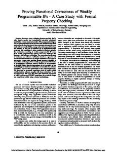
object p p p p p p
op lock() RET unlock() lock() RET RET
thread A A A B B A
Figure 8: An example history involving two threads. 2.7.3
Linearisability
Linearisability [8] is a property of certain modules that allows concurrent use of the module functions to be reduced to a sequential application of the same operations. This allows complicated assertions and proofs about concurrent programs to be reduced to ones about their sequential equivalents. Intuitively, a module with the linearisability property guarantees that none of its operations will expose “in progress” state to other threads observing the module. The original formal definition of linearisability is given in terms of a “history” H. A history describes the execution of a piece of code in terms of a sequence of call and return events in different threads. Note that a call may take effect before its return event is registered. For example, fig.8 describes an execution of a program where thread A locks and unlocks the lock p but B is able to lock the lock before A returns, but presumably after A’s unlock has changed the lock’s state. A history is “sequential” if it begins with a call, and every call is immediately followed by its response without anything in between. Fig.8 is an example of a “concurrent” history, where this condition is not met. Herlihy uses linearisability to describe a correctness condition for modules which may be used in a concurrent setting. Roughly, a module is “correct” if every possible history made up of its operations is linearisable. This is equivalent to proving that every module operation has exactly one distict atomic time point at which it appears to take effect, its “linearisation point”. [9]
2.7.4
Abstraction and abstract atomicity
Whether or not we consider an operation on a module to be atomic can depend on the granularity at which threads observe the module’s state changes [10]. We can give a specification for a module in terms of a state transition system.
22
For example, a lock could be described by the set of states {0, 1}. The lock operation could be described by the transition 0 1 and the unlock operation could be described by the transition 1 0. Roughly, if we can show that an implementation of either of these operations has a unique time point (the linearisation point) at which its transition occurs, we can treat this operation as atomic, since threads inspecting the state of the lock can only see the state before or after the transition (there is no intermediate or “working” state). Consider the counter module described previously. Naively, its set of states is N, the set of natural numbers. Its incr operation embodies the transition n n + 1 for some n that is related to the value of the counter at the time the function is called (this is an awkward caveat, but one we will do away with later). Consider an extension of the counter with the operation incrTwo, which we implement by calling incr twice sequentially. Under the current setup, we cannot consider incrTwo an atomic operation; other threads inspecting the value of the counter will see multiple states depending on how far incrTwo has executed. There is no simple “before” and “after” point that the operation can be described in terms of. Now, we will perform the crucial trick. We can wrap the counter in another level of abstraction. Let us define another module, “outerCounter”. The outerCounter module has two states: (0) and (> 0), which can be read as “the counter is equal to 0” and “the counter is greater than 0”. The incr operation for the counter module is also an operation over the outerCounter module. It will perform one of the two transitions (0)
(> 0)
(> 0)
(> 0)
but crucially, it will perform exactly one (if it terminates), and therefore we can still treat incr as atomic. The (> 0) (> 0) transition, which does not change the state, is what is known as an “abstract skip”. Any thread inspecting the state of outerCounter will not be affected as a result of the abstract skip occurring, so we can always choose whether or not to count it as a linearisation point. What about incrTwo? The first incr operation will perform one of the two transitions above, however the second incr will always be an abstract skip. Therefore we can consider the incrTwo operation as performing exactly one transition, and therefore it is an atomic operation for the outerCounter module.
23
incr(x); incr(x); v := read(x); if (v > 1) { critical } Figure 9: A trivial program that must execute critical. There are a few important points to make here. Any code that can be proven to implement the original counter module can also be proven to implement the outerCounter module. However, the discussed implementation of the incrTwo operation can only be considered atomic so long we only reason about the behaviour of every thread in terms of the outerCounter state system. This is important since proving that all the operations of a module behave atomically gives us the linearisablity correctness result as discussed above. For a counter module with incrTwo implemented as two incr calls, we can either give incrTwo a non-atomic specification, and break the linearisablity of the whole module, or we can abstract our view of the state system to the point that incrTwo appears linearisable. Obviously for this contrived example, the abstraction is hideously inexpressive (since incr would only guarantee to take the state of the module to (> 0), we could not even prove that the code of fig. 9 executes critical ), but it does motivate that different levels of abstraction give us different guarantees about the atomicity of operations. Many modern program logics provide ways of encoding the abstract atomicity of an operation. However, there are several different approaches. Iris [11] can reason about the abstract atomicity of an operation using higher order specifications. A history-based approach [12] proves abstract atomicity by reasoning about “subjective” histories. We will concentrate on a system which gives a direct, first-order specification for abstractly atomic operations; TaDA.
2.8
TaDA
TaDA (Time and Data Abstraction) [13] is a program logic which combines the expressive assertions of separation logic with notions of abstract atomicity, in order to prove “atomic specifications”. An operation with an atomic specification can be treated as though it executes in a single “step”. This is like the
24
linearisability previously discussed. Atomic specifications are expressed using triples”. D “atomic E D E In its simplest form, the atomic triple is written ` x ∈ X. P (x) C Q(x) . The meaning of the triple is most intuitively explained using the following diagram. A
P
PQ
start
linearisation point
terminates
To explain, an atomic triple expresses that C contains exactly one linearisation point. P and Q are assertions about the state of shared memory. The precondition P expresses that P will hold from when C begins execution until its linearisation point. P is parameterised by x, which may vary within the set X up until the linearisation point. The pseudo-quantifier (or “funny for-all”) to the left of the assertion is the syntax for this. When the linearisation point occurs, C will atomically update from P to Q, and Q can use x to refer the the value of x immediately before the linearisation point. After the linearisation point, C guarantees not to alter shared state any more, but makes no guarantees that Q will remain true (other threads could invalidate it). P may describe a set of possible states, either because it directly describes a disjunction of several potential states, or because of the pseudo-quantified x. The environment is free to alter the shared memory described by P so long as it remains within the set. For now, since we are describing partial correctness, all bets are off if C fails to terminate. It important to stress that property embodied here is abstract atomicity. It is possible to describe updates to shared memory at various levels of granularity, only some of which may appear to be abstractly atomic. It will now be shown how TaDA formalises atomic update and these different levels of abstraction.
2.8.1
Formalising an atomic update
TaDA owes much to the formalism of CAP, using predicates to abstract ownership (and more generally, the existence) of particular resources. For example, a lock may be described by the abstract predicate L(r, x, s), with s ∈ {>, ⊥}. x is, again, the memory location of the lock. r is a parameter which uniquely identifies certain internal components of the module. In some older papers it
25
was elided, making the logic subtly unsound. A simple atomic specification for unlock might look something like the following. D E D E ` L(r, x, >) unlock L(r, x, ⊥) Such a specification is only possible due to the unique guarantees of the atomic triple. A non-atomic specification could not have this post-condition, as it would have to account of the possibility of the lock being re-locked before unlock function returns. The atomic specification for lock is more complicated, and makes use of the pseudo-quantifier. D E D E ` l ∈ B. L(r, x, l) lock(x) L(r, x, >) ∧ ¬l A
B is the set of booleans. Because of the pseudo-quantifier, we have encoded that the environment is allowed to arbitrarily lock and unlock the lock until the linearisation point occurs. The ¬l condition in the post-condition enforces that the lock must have been unlocked immediately before the linearisation point (which is when lock actually locks the lock). To prove these specifications against an implementation, it is necessary to provide an interpretation (, definition) for the abstract predicate. This is done in terms of “regions” and “guards”, which further abstract the shared memory underlying the predicate. A region describing the memory of a lock might look something like Lock(x, s) with s ∈ {0, 1}. Regions are associated with a set of states, and a state transition system that defines the atomic updates that can be made. Here the set of states for Lock are {0, 1}, and the transition system is as follows. G : 0 1 G : 1 0 The gist here is that to prove an atomic specification for an implementation of unlock, we must show that its code makes exactly one of the transitions here across the entire execution of the function. The G parameterisation of the state transition is the “guard”. A transition is only allowed if the correct guard is held in the precondition. We will see the power of this later, but for Lock, every transition will be guarded by the same guard, G. The interpretation of L in terms of Lock is close to trivial here, but this is not always the case. It is provided in fig. 10. Since multiple regions of the same type may be present, the region and its associated guard are given a unique “region identifier” a. The 26
L(a, x, ⊥) , Locka (x, 0) ∗ [G]a L(a, x, >) , Locka (x, 1) ∗ [G]a Figure 10: Interpretation of L(a, x, s). guard is included in the interpretation to encode that holding the predicate means that the thread has permission to perform the region’s transitions. In general this is not always the case. Proving that a specific line of code executes an action in a region’s transition system involves the use of two rules which can be considered the powerhouses of TaDA; “make atomic” and “update region”.
2.8.2
Make atomic
The TaDA paper initially explains the make atomic rule using a simpler variant which is reproduced in fig. 11. This rule is TaDA’s instrument for proving that a block of code can be considered abstractly atomic. We are allowed to conclude that C can be described by an atomic triple updating , if we are able to prove the following;: • C performs exactly one update to the region ta (x). • The local thread holds the correct guards for this action. . The first restriction is enforced by the unfulfilled “atomicity tracking component” a Z⇒ �. The state of a region with region id a may only be altered locally by non-atomic code through the “update region” rule, which requires an unfulfilled atomicity tracking component in the precondition, and produces a “fulfilled” atomicity tracking component which records the transition. Since these tokens are only generated once within a make atomic, we can be sure that only one update has occurred. The second restriction is enforced by the top antecedent. Tt (G) defines the set of transitions allowed by the guards G. We pick a subset of these allowed transitions and stick them on the left hand side of the turnstile in a place known as the “atomicity context”. The update region rule will only allow a transition that is contained in the atomicity context. Let us consider the proof of a simple implementation of unlock given in fig. 12, given in an elaborated sketch style. The “abstract; quantify a” line unwraps the abstract predicate into its interpretation. The make atomic rule prepares the unfulfilled atomicity
27
{(x, y) | x ∈ X, y ∈ Q(x)} ⊆ Tt (G)∗ � � � � ∃x ∈ X. ta (x) ∃x ∈ X, y ∈ Q(x). Q(x) ` a:x∈X C ∗ a Z⇒ � a Z⇒ (x, y)
�
� ` x ∈ X. ta (x) ∗ [G]a C ta (Q(x)) ∗ [G]a A
update region
make atomic
abstract
Figure 11: Simplified make atomic.
� L(a, x, >)
� Locka (x, 1) ∗ [G]a 0` a :�1 Locka (x, 1) ∗ a Z⇒ �
� x 7→ 1 [x]
:= 0;� x 7→ 0
� a ⇒ Z (1, 0)
� Lock�a (x, 0) ∗ [G]a
L(a, x, ⊥) Figure 12: Proof of unlock(x). tracking component, and adds the action to be fulfilled to the atomicity context. Executing the line “[x] := 0;” satisfies the action and therefore fulfills the atomicity tracking component. The make atomic rule can now update the region since we have concluded with a fulfilled atomicity tracking component.
2.8.3
The full TaDA triple
The generalised form of the TaDA atomic triple contains not just information about the state of shared memory, but also “private state” assertions. D E D E ` x ∈ X. pp P (x) C y ∈ Y. qp (x, y) Q(x, y) E
A
Here is a visual representation of the transformation of the private state over the course of the execution of C. The private and public parts of the assertions are separated by a vertical bar. The right hand side is the old assertion we discussed before. The left
28
P
PQ
pp start
p0p p00p linearisation point
qp terminates
hand side of the assertion is called the “private” part. Its meaning is slightly different. Assertions may only be put on the private side if they are stable against anything the environment may do. This is defined by the transition system of the various regions. If the local thread does not have exclusive permission to perform actions on the region it is making an assertion over (for example if the region’s actions are predicated by guards that other thread’s might hold) then the private state cannot contain any assertion that could be invalidated by this action taking place. In the lock example, other threads can possibly hold the guard G, so the private side of an assertion could never contain the assertion Lock(x, 0), since another thread could lock the lock and invalidate this.
2.8.4
The non-atomic triple
In TaDA, triples of the form {P } C {Q}, which specify the execution of a nonatomic C, are purely syntactic sugar for the atomic triple hP | >i C hQ | >i. The assertion effectively states that we have no information at all about linearisation points that occur during the execution of C, and that the assertions P and Q, being in the private side, must be fully stable against any possible region updates. This mirrors a rely-guarantee style stability condition, except the actions the assertions must be stable with respect to are determined by which guards are held locally and the transition systems of the regions.
2.8.5
Update region
The final question is how TaDA ensures that a piece of code satisfies the atomicity tracking component. To fully explain this, we must introduce the concept of “region interpretations”. Like an abstract predicate, a region can be “opened up” to reveal a lower level representation. However, this is done in a far more restricted fashion. A region may only be opened for a single atomic update, after which it is closed again. This ensures that other threads with access to the region will never observe it in the middle of an update. See fig. 13 for an example. Several rules will reference the region interpretation function 29
I(Locka (x, 1)) , x 7→ 1
I(Locka (x, 0)) , x 7→ 0
Figure 13: Example region interpretation. � ∃z ∈ Q(x). I(tλa (z)) ∗ q1 (x, y, z) y ∈ Y. qp (x, y) ∨ I(tλa (x)) ∗ q2 (x, y)
λ+1 � x ∈ X. pp ta (x) ∗ p(x) ∗ a Z⇒ � C � � Q(x), A ` ∃z ∈ Q(x). tλ+1 (z) ∗ q (x, y, z) ∗ a ⇒ Z (x, z) 1 a y ∈ Y. qp (x, y) ∨ tλ+1 a (x) ∗ q2 (x, y) ∗ a Z⇒ � �
E
A
λ, A `
� � λ x ∈ X. pp I(ta (x)) ∗ p(x) C
A
E
λ + 1, a : x ∈ X
Figure 14: The update region rule. I, which need only needs to be defined if the region is opened directly in the proof. The full update region rule is give in fig. 14. This also introduces the last annotation to the left hand side of the turnstile: the “level”. A region can only be opened (via the region interpretation function) if the proof is at the same level of the region (tλa (x) where λ is the region’s level). The proof’s level then decreases by one. This ensures that regions defined in terms of each other cannot be opened in an infinite loop, which would be unsound. In many proof sketches the level will be elided, since it is only important if the proof contains a recursively defined region. Note that update region must be able to handle both the case where the linearisation point occurs, and the case where it does not. This is represented by the disjunction in both the antecedent and consequent of the update region rule. In the case where the update is a simple memory cell mutation, the “didn’t happen” case is trivially false. However this is not the case when the update is a CAS, as can be seen in the lock proof of fig. 15. Notice how the two cases of the CAS neatly mirror the two cases of the update region rule. Once the loop terminates, we know that the CAS has succeeded, and therefore that the region has been updated and the linearisation point has occurred.
2.8.6
Proving a client
TaDA’s expressivity comes from its ability to layer abstractions. Interpretations of regions and abstract predicates are permitted to contain further regions and abstract predicates which represent memory at a lower level. In this way, the 30
A
l ∈ B. � L(a, x, l) �
y ∈ {0, 1} . Locka (x, y) ∗ [G]a 1∧y =0` a :�y ∈ {0, 1} ∃y ∈ {0, 1} . Locka (x, y) ∗ a Z⇒ � do�{ ∃y ∈ {0, 1} . Locka (x, y) ∗ a Z⇒ � update region
make atomic
A
abstract; y := if l then 1 else 0
A
n ∈ {0,� 1} . x 7→ n b � := CAS(x, 0, 1); � (x 7→ 1 ∧ n = 0 ∧ b = 1) ∨ (x 7→ n ∧ n 6= 0 ∧ b = 0)
� � ∃y ∈ {0, 1} . Locka (x, y) ∗ (a Z⇒ (0, 1) ∧ b = 1 ∨ a Z⇒ � ∧ b = 0) }� while (b = 0); a Z⇒ (0, 1) ∧ b = 1 �
Locka (x, 1)
� ∗ [G]a ∧ y = 0 L(a, x, >) ∧ ¬l Figure 15: Proof of lock(x) state space of a higher level region can offer an abstracted or subsetted view of the behaviour of a lower one. Let us look at a concrete example, which will also serve to illustrate TaDA’s weakening rules for using atomic code as part of a non-atomic program. The TaDA style specification for a counter module is given below. Note that the client does not need to know about the interpretations used to prove the counter implementation. D E D E ` n ∈ N. C(a, x, n) read(x) C(a, x, n) ∧ ret = n D E D E ` n ∈ N. C(a, x, n) incr(x) C(a, x, n + 1) ∧ ret = n D E D E ` C(a, x, n) wkincr(x) C(a, x, n + 1) ∧ ret = n A A
Note that for wkincr, the lack of pseudoquantifier indicates that this specification will only hold when the operation is executed in an environment where the value of the counter does not vary, i.e. where there are no concurrent increments occurring.
31
We will prove that the following clients both increment an initially zero-valued counter to exactly two.
2.8.7
A sequential client incr(x); incr(x);
We will define a thin wrapping region for C in the client, the only effect of which will be to encode that no other thread has permission to increment the counter. Let us call this region CCounter. The transition system and guard algebra for the client is as follows: ∀n ∈ N. H : n
n+1
H•H=⊥
The equivalence H • H = ⊥ encodes that if one thread holds H, no other thread can, since their composition is equal to ⊥. A consequence of this is that the guard cannot be split; H ⇒ H ∗ H does not hold. This means that if we hold [H] in a non-atomic assertion, we do not need to worry about stability with respect to transitions guarded by [H], since no other thread can make them. The region interpretation of CCounter is as follows: I(CCountera (r, x, n)) , C(r, x, n) We define an abstract predicate to represent the client at the counter level, CC. Its only effect is to encode the client’s view of its exclusive permission to the counter. The interpretation of CC is as follows: CC(a, r, x, n) , CCountera (r, x, n) ∗ [H]a Now we can proceed with the proof, which can be found in fig. 16. Note that if [H] could be held by another thread, the non-atomic line {CCountera (r, x, 1) ∗ [H]a } would not be stable since other regions could increment the counter, and would have to be weakened to {∃n ≥ 1. CCountera (r, x, n) ∗ [H]a }, destroying the proof.
32
use atomic
weaken
abstract
use atomic
CC(a, r, x, 0) � CCounter (r, x, 0) ∗ [H] a a �
CCountera (r, x, 0) ∗ [H]a
� C(r, x, 0) incr(x);
� C(r, x, 1) �
CCounter (r, x, 1) ∗ [H] a a � CCounter a (r, x, 1) ∗ [H]a �
CCountera (r, x, 1) ∗ [H]a
� C(r, x, 1) incr(x);
� C(r, x, 2)
� CCountera (r, x, 2) ∗ [H] � a CCounter � a (r, x, 2) ∗ [H]a CC(a, r, x, 2) weaken
�
Figure 16: Sequential counter client proof 2.8.8
A concurrent client incr(x);
incr(x);
We will define a client region CCounter’ which tracks the updates of each branch separately. Its states will be tuples of (n1 , n2 ). The state transition system and guard algebra are as follows. ∀n, n0 ∈ N. J : (n, n0 ) H=J•K
(n+1, n0 )
∀n, n0 ∈ N. K : (n, n0 )
J•J=⊥
(n, n0 +1)
K•K=⊥
This guard algebra encodes that each branch will take exclusive permission for updating one half of the “counter”. The region interpretation of CCounter’ is as follows. I(CCounter0 a (r, x, n, n0 )) , C(r, x, n + n0 ) The client’s abstract predicate CC0 will be as interpreted as follows: CC0 (a, r, x, n + n0 ) , CCounter0 a (r, x, n, n0 ) ∗ [H]a 33
� 0 CC (a, r, x, 0) � 0 CCounter (r, x, 0, 0) ∗ [H] a a � 0 0 � 0 CCounter0 a (r, x, 0, 0)0 ∗ CCounter � a (r, x, 0, 0) ∗ [J]0 a ∗ [K]a ∃n . CCounter a (r, x, 0, n ) ∗ [J]a ∃n. CCounter a (r, x, n, 0) ∗ [K]a 0
n ∈ N. �
n ∈ N. � 0 0 CCounter a (r, x, 0, n ) ∗ [J]a CCounter0 a (r, x, n, 0) ∗ [K]a
�
� C(r, x, n0 ) C(r, x, n) incr(x);
incr(x); 0 �
� C(r, x, n + 1) C(r, x, n + 1) �
�
0 0 CCounter0 a (r, x, n, 1) ∗ [K]a � 0 CCounter 0a (r, x, 1, n 0) ∗ [J]a � ∃n� . CCounter a (r, x, 1, n ) ∗ [J]a ∃n. CCounter0 a (r, x, n, 1) ∗ [K] a 0 0 0 0 ∃n, n . CCounter (r, x, n, 1) ∗ CCounter (r, x, 1, n ) ∗ [J] ∗ [K] a a a a � 0 (r, x, 1, 1) ∗ [H] CCounter a � 0 a CC (a, r, x, 2) use atomic
weaken
use atomic
weaken
abstract
A
A
Figure 17: Parallel counter client proof The proof of the concurrent client can be count in fig. 17. Notice how each individual thread loses information about the other thread’s contribution when it only holds its own guard. The region assertions maybe be split freely as seen in the non-atomic lines immediately before the parallel rule, since holding one does not give permission to modify it; this is the job of the guard. After the parallel rule, we know that there is only one possible state of the CCounter’ region given each thread’s knowledge and the guards we hold. While the client region defined here is very targetted towards proving this example, note that we are still able to use the general form of the module’s specification. This is a key power of TaDA. By layering regions and predicates on top of each other, “gimmicky” formalisms may augment more general ones precisely where they are needed by a client’s proof, instead of having to introduce them at the level of the module specification.
2.9
Total correctness
As stressed previously, all of the systems described so far only prove partial correctness with respect to a specification. The program the proof is conducted over may loop or recurse infinitely, and in this case the proof makes no guarantees about its behaviour. Termination is a useful property, so it makes sense to 34
x := 10; while (x > 0) { x := x − 1; }
x := 10; while (1) { x := x − 1; }
Figure 18: Two trivial while programs. The first program can be proven to terminate. try and prove it! Of course trying to build a proof system that decides the halting problem is doomed to failure (leaving aside that partial correctness is also undecidable in general!), so existing systems severely restrict the space of provable programs.
2.9.1
Loop variants
Take a trivial while programming language with no recursion or parallelism. Now the only way a program can fail to terminate is if a loop never has its condition falsified. Our aim is therefore to find a variant for every while loop; a value on a finite decreasing chain that decreases with each loop iteration [14]. If such a value is found, then the loop must terminate, since the value cannot decrease infinitely. See fig. 18 for examples. In the first example, v forms a variant for the while loop, since v ≥ 0 is an invariant of the loop and v decreases each iteration. In the second example, even though v decreases each iteration it is not a variant since it will not decrease finitely. This system is very neat, but clearly restricting ourselves to such a language is not satisfactory.
35
� � ∀γ ≤ α. λ; A `τ P (γ) ∧ B C ∃β. P (β) ∧ β < α � � λ; A `τ P (α) while (B) C ∃β. P (β) ∧ α ≥ β ∧ ¬B Figure 19: The while rule of Total TaDA
� � assign ∀γ ≤ 10. `τ x = γ x := x − 1 x = γ − 1 � � f rame, cons ∀γ ≤ 10. `τ 0 < x ≤ 10 ∧ x = γ x := x − 1 ∃β. 0 ≤ x ≤ 10 ∧ x = β ∧ β < γ � � while Loop : `τ 0 ≤ x ≤ 10 ∧ x = 10 while (x > 0) x := x − 1 ∃β. 0 ≤ x ≤ 10 ∧ x = β ∧ 10 ≥ β ∧ x ≤ 0
� � assign, cons `τ emp x := 10 x = 0 ∧ 0 < x ≤ 10 Loop sequence, cons � � `τ emp x := 10; while (x > 0) {x := x − 1} x = 0 Figure 20: An instance of the while rule with an instantiated (in)variant.
2.10
Total TaDA
The notion of loop variants can be extended into the concurrent language of TaDA. Total TaDA [15] is an extension to TaDA which proves total correctness. A triple in the Total TaDA system has the same meaning as in TaDA, with the added guarantee that C will terminate. There are two ways in which a statement in the language of TaDA can fail to terminate; bottomless recursion, and while loops which never have their condition invalidated. The added complication is that, since TaDA is a concurrent language, a while loop condition may be affected by the actions of other threads. In some circumstances, it is still possible to determine a variant for the loop, except now other threads may be the ones causing it to decrement. The Total TaDA while rule is given in fig. 19. The P (γ) assertion describes a loop invariant P which is parameterised by a variant γ which decreases each time the body is executed. A proof of the termination of a simple while loop program is given in tree style in fig. 20. Notice that the invariant contains the assertion x = γ, which forms the variant for the loop. The initial value of the variant, α, is set to 10. Now we will look at a more complicated example, where the variant of the loop is decreased as a result of actions by the environment, not just the local thread.
36
2.10.1
Termination of increment
Consider the counter example described previously. For convenience, the incr function is reproduced below. function incr(x) { b := 0 while (b = 0) { r := [x]; b := CAS(x, r, r + 1); } return r; } We previously discussed aD (partial)Especification D for this function in TaDA; E incr would be ` n ∈ N. C(r, x, n) incr(x) C(r, x, n + 1) ∧ ret = n . To prove that the above implementation satisfies this specification, we must give an interpretation of the abstract predicate where the states of the counter are the natural numbers, and incr embodies the transition n n + 1. A
Now we must consider total correctness. Intuitively, what is the termination condition for the loop? So long as only a finite number of increments run in parallel, eventually the CAS will succeed and the loop will terminate. This is because the CAS will only fail if at least one of the incr calls succeeded in modifying the counter, thus terminating. Eventually either our local CAS will succeed, or every other incr call will succeed first, but then we are guaranteed to succeed immediately after. This arrangement can be thought of in terms of a “global variant” across the entire counter module. Call the number of n n + 1 operations allowed to occur α. Each time we iterate around the loop, there are two possibilities. Either we succeed, decreasing α by 1, or our CAS fails, which means another n n + 1 operation has occurred since our last loop iteration, and α must have decreased by 1. Clearly there cannot be an infinite number of increments in parallel, since we would run out of α. We can encode this intuition into our abstract predicate and counter region. Now the counter predicate will be parameterised by an ordinal number which, as long as it is greater than 0, provides permission to increment the counter. This is enforced by the underlying region’s transition system.
37
The interpretation of the counter predicate C is as follows: C(r, x, n, α) , Counterr (x, n, α) ∗ [G]r The region’s transition system is defined as follows: ∀n, m ∈ N, α > β. G : (n, α)
(n + m, β)
This forces any action incrementing the counter to decrease the ordinal. The region interpretation is defined as follows: I(Counterr (x, n, α)) , x 7→ n
38
A
open region
� x 7→ n ∧ γ ≥ α > β(n, α)
v := [x]; � x 7→ n ∧ v = n ∧ γ ≥ α > β(n, α) ∧ (n > v ⇒ γ > α)
∃n, α. Counterr (x, n, α) ∗ r Z⇒ � ∧ γ ≥ α > β(n, α) ∧ (n > v ⇒ γ > α)
update region
make atomic
�
�
A
abstract
∀β. n ∈ N, α � C(r, x, n, α) ∧ α > β(n, α) � Counterr (x, n, α) ∗ [G]r ∧ α > β(n, α) (n + 1, β(n, α)) r� : (n, α) ∧ n ∈ N ∧ α > β(n, α) `τ ∃n, α. Counterr (x, n, α) ∗ r Z⇒ � ∧ α > β(n, α) b � := 0; ∃n, α. Counterr (x, n, α) ∗ r Z⇒ � ∧ b = 0 ∧ α > β(n, α) while (b = 0) { ∀γ � ∃n, α. Counterr (x, n, α) ∗ r Z⇒ � ∧ γ ≥ α > β(n, α)
n∈N � x 7→ n ∧ γ ≥ α > β(n, α) ∧ (n > v ⇒ γ > α) � b := CAS(x, v, v + 1); � α > β(n, α) ∧ if b = 0 then γ > α ∧ x 7→ n else γ > α ∧ x 7→ n + 1 ∧ v = n
� ∃n, α. γ ≥ α > β(n, α) ∧ if b = 0 then Counterr (x, n, α) ∗ r Z⇒ � ∧ γ > α) else r Z⇒ (v, α), (v + 1, β(n, α))
}� ∃n, α. r Z⇒ (n, α), (n + 1, β(n, α)) ∧ v = n return v; � ∃n, α. r ⇒ Z (n, α), (n + 1, β(n, α)) ∧ ret = n
� Counter (x, n + 1, β(n, α)) ∗ [G] ∧ ret = n r r
� C(r, x, n + 1, β(n, α)) ∧ ret = n
Figure 21: Total correctness of incr.
Now, we can proceed with the proof of termination. It is given in fig 21. The line v := [x]; allows us to establish a known value for the ordinal. We can relate this value to the value of the ordinal at the point of the CAS. If the CAS fails, we know that a further increment operation must have occurred in the environment since the read. This means we have proven that the ordinal decreases, even if we do not succeed in the update on this iteration. The reason we prove the specification for all functions β with α > β(n, α) is so that the client calling incr can choose how much to decrement the ordinal by. The 39
x := makeCounter(); m := random(); while (m > 0) { incr(x); m := m − 1; } Figure 22: A non-deterministic number of increments. client can only perform a finite number of increments, since they are forced to strictly decrease α every update. The reason ordinal numbers are used, rather than merely the natural numbers, is because this allows to handle non-deterministic numbers of calls. For example, the environment could execute a non-deterministic but finite number of increment actions, and incr would still guarantee to terminate. The Total TaDA paper gives the example of a loop which executes a random number of iterations which is reproduced in fig. 22. Since the value of the the abstract predicate’s ordinal must be chosen at the point of the object’s creation, there is no natural number we can pick which would allow us to fulfil our proof obligations that we always have enough “fuel” left to execute the increment inside the loop. The correct solution is to choose the initial value of the counter’s ordinal to be ω, the “first uncountable ordinal”. The proof rule of fig. 19 requires us to prove the body ∀γ (where γ will be an ordinal related to the variable m, our variant). Our specification for incr allows us to choose any β we want to decrement the ordinal, i.e. the client has complete control over how much the ordinal should be decremented. In the case that the counter ordinal is equal to ω, it can be decremented to m − 1 as a result of the call. Otherwise, it can be decremented by 1, since every ordinal number less than ω is a natural number. Total TaDA is a surprisingly neat and compact extension to TaDA which can prove total correctness. However it must restrict itself to a certain subclass of concurrent programs, namely those which are “lock-free”. It is arguable that the programs for which a termination result would be most valuable lie outside this class.
40
2.11
Total correctness: blocking algorithms
Herlihy characterises concurrent programs according to their termination conditions [16]. Each condition forms an axis along which the space of concurrent programs may be subdivided. A concurrent program or algorithm is one that executes across multiple threads simultaneously. Herlihy gives formal classification of the progress of these threads in terms of histories (as mentioned previously). Since the details of his formalisation are orthogonal to those of TaDA, his classifications will be explained intuitively.
2.11.1
Maximal vs minimal progress
If at least one thread of a concurrent program is guaranteed to be “working” at any time, the program is characterised as making “minimal progress”. If no thread can be indefinitely prevented from working, this is “maximal progress”. An (extreme) example of a program characterised by maximal progress would be one where no threads access shared memory, and only perform local calculations which terminate. An example of minimal progress is the concurrent incr implementation used as an example in previous sections. At least one concurrent call to incr is guaranteed to succeed, but this may cause other threads to experience delay as they may have to execute an extra loop iteration in their own calls. In the setting of Total TaDA, where we have a local proof and a stability condition abstracting all other threads as a nebulous “environment”, we characterise operations as causing delay if they decrease the ordinal of their region, since this is our way of enforcing that such delay must be finite. incr causes delay, but read does not. In the Herlihy setting, this means that a concurrent program with multiple increments in parallel only guarantees minimal progress.
2.11.2
Blocking vs non-blocking
A blocking algorithm is one in which some thread may be unable to execute until another thread makes an “unblocking action”. In particular, it may be the case that the thread would not terminate if it were executed in isolation. If no thread can experience this, the algorithm is “non-blocking”.
41
function lock(x) { b := 0; while (b = 0) { b := CAS(x, 0, 1); } }
function unlock(x) { [x] := 0; }
Figure 23: A spin lock implementation. function lock(x) { t := incr(x.next); v := 0; while (v < t) { v := read(x.owner); } }
function unlock(x) { incr(x.owner); }
Figure 24: A ticket lock implementation. Total TaDA has no mechanism for modelling blocking actions/threads/algorithms. Any operation that can be proven to terminate in Total TaDA is necessarily non-blocking.
2.11.3
A periodic table of programs
Herlihey gives classifications to algorithms based on which combination of the previous attributes they exhibit (his original paper defines a class in between blocking and non-blocking, but this is uninteresting to us since it depends on properties of the OS scheduler, which is not modelled in TaDA). maximal minimal
non-blocking wait-free lock-free
blocking starvation-free deadlock-free
Program classes which guarantee minimal progress are a superset of their maximal progress equivalents. From this we can see that Total TaDA handles the lock-free class of concurrent program. A deadlock-free module operation only guarantees termination if the environment guarantees to only perform a finite number of operations during its local execution. Otherwise, the environment could continue to do work infinitely, satisfying the definition of minimal progress without the local operation ever 42
[v] := 0; b := 0; while (b = 0) { lock(x); unlock(x); b := [v]; }
lock(x); unlock(x); [v] := 1;
Figure 25: Terminates if lock is starvation free. finishing. Furthermore, since it is blocking, the environment must terminate in an “unblocked state” which allows the operation to finish if it has not already. Spinlock is an example of a deadlock-free module. A possible implementation is given in fig. 23. We can see that if the local thread is running lock, it will only terminate if the environment only performs a finite number of lock operations itself, since otherwise the local thread’s CAS could fail forever. Furthermore, the environment must eventually leave the lock in an unlocked state. Ticket lock is an example of a starvation-free module (assuming the counters it uses are wait-free). An implementation is given in fig. 24. Even if the environment is running an infinite number of lock-unlocks, eventually owner will increment to the value of next that was read at the start of the local thread’s lock operation. The environment still needs to guarantee it will always release a held lock, however. Fig. 25 is an example of a client program that guarantees to terminate using ticket lock, but not with spinlock. The aim of this project is to extend Total TaDA to handle programs from the deadlock-free class. We will first examine arguably the two most prominent logics that reason about the termination of deadlock-free programs, and discuss both the lessons that can be learned from them, and the significant compromises made by the existing work.
2.12
LiLi
Lili [17] is a rely guarantee style system which incorporates the separating conjunction of separation logic, and certain aspects of linearisability from
43
Herlihy’s work to prove termination of module operations. There are a few key concepts in LiLi that are relevant to our proposed extension.
2.12.1
Definite actions
LiLi judgements enforce that a thread will carry out a set of “definite actions” as part of its execution. In turn, it relies on the environment carrying out a set of definite actions in order to guarantee its own termination. For example, a thread may be required to fulfill the definite action (L 7→ 1) (L 7→ 0) which encodes that if it ever locks the lock L, it must release it. Unfortunately, LiLi’s reasoning requires that the exact thread ID currently holding the lock is encoded somewhere inside the resource’s state, so in a real proof the definite action might look something more like (L 7→ t) (L 7→ 0) where t is a thread id. This means that LiLi can only abstract the environment in a limited way since the number of threads must be fixed in advance of the proof.
2.12.2
Unblocking conditions
A loop inside a blocking program will not have a variant. For instance, this is the loop of a spin lock implementation (with the lock at location x). b := 0 while (b = 0) { b := CAS(x, 0, 1); } If the lock is locked, the CAS will never succeed, and therefore the loop will never terminate. However, if the lock is unlocked, the loop is guaranteed to terminate. We can say that L 7→ 0 is the “unblocking condition” of the loop. The loop is guaranteed to terminate if this condition is established and preserved. Since the local thread knows the actions any other threads are guaranteed to make (via the definite actions) it is possible to reason that the unblocking condition is inevitably established.
2.12.3
Limitations
As mentioned, LiLi’s assertions about the actions of the environment are explicitly parameterised by thread IDs. This is anathema to TaDA’s more 44
abstracted view of the environment. It seems intuitive that we must have some sort of formalisation of what the environment must do to guarantee local termination, as opposed to just what it may do. However, LiLi solves this problem by reasoning about a ordered, finite queue of actions by each thread. There are more fundamental mismatches between the goals of LiLi and Total TaDA. LiLi aims to solve a far simpler problem - namely that the operations of a module terminate and appear linearisable. In this way, LiLi’s correctness condition is much like Herlihy’s original linearisability condition. LiLi cannot provide a lock specification that a client can use to reason about its own termination, since it provides no mechanism for a client to verify that it satisfies the lock operation’s required definite actions. In fact, the language of LiLi does not include function calls at all! Even within a module operation proof, references to lock and unlock calls are merely typographical shorthand for an inlined loop or similar series of statements which functions as a lock. Furthermore, LiLi’s style of reasoning scales poorly if the operations of a module do not all perform the same blocking actions. Every substantial proof in the paper is of a module embodying some variation of a counter increment or list push/pop, which is implemented as a critical section surrounded by some flavour of lock-unlock. This is a very local style of blocking, since no module operation can terminate without unblocking every other operation. We will see in general that this is not the case.
2.12.4
Lessons
The way the language of Total TaDA blocks is similar to the way LiLi blocks - a while loop condition which relies on another thread/the environment performing an update. It seems intuitive that we will have to determine the loop’s unblocking condition, and guarantee that the environment performs actions that eventually satisfy and preserve it. However, LiLi’s formalism offers us no help in doing this, since the sacrifices they have made to ensure their rules are sound (no clients, no thread forking, no function calls, poor non-local blocking) constrict their expressivity to the point that porting their restrictions into the world of TaDA would leave us with almost no logic at all, due to the way TaDA is built to facilitate modular proofs.
45
2.13
Bostr¨ om and M¨ uller
This work [18] offers a far more complete logic with fewer odd restrictions. However, their memory model is based on message passing, and does not include a shared heap. This means that all inter-thread blocking is mediated by language primitives. The only way for any thread to wait on the update of another is through the lock, (channel) receive and (thread) join operations, which are given as part of the semantics of the language and not as module specifications. In this way, it is impossible for a thread to experience arbitrary blocking that is not mediated through one of these constructs. Because of this, it is possible to build a bespoke “token language” for each construct. For example, a lock operation produces a “releases” obligation token that must be consumed by a corresponding unlock, while a receive operation on a channel must either consume a “sends” credit token produced by an earlier send to the channel, or produce a sends obligation token, representing that it is blocking on a send that may not have occurred yet. 2.13.1
Lessons
Separation logic in general is based on a model with a shared heap, so any module can potentially block in a way that is not possible with a message passing setup. The equivalent to their approach in Total TaDA would be that specifying a module for use by a client also means specifying a token language to go with it, which describes exactly how it blocks (in some way this would be analogous to the existing guard tokens, which abstract both the thread’s and the environment’s permission to update the region). However, the fundamental nature of Total TaDA’s assertions means that this technique would almost certainly be unsound, since P ∗ Q ⇒ P is always sound; i.e. we could forget tokens whenever we want, even if they denote an obligation to unblock.
3
B-TT: extending Total TaDA
We want to show that every possible execution of a blocking program terminates. We can view each execution as a trace of updates to shared state, but in particular we only care about updates to module instances which might be
46
involved in blocking. Take the following code as an example: α1 lock(x); α2 lock(x); unlock(x); β α3 unlock(x); Every real execution of this code can be characterised by some sequence of the timestamps marked in red. Indeed, because of the way lock blocks, there is only one possible sequence: α1 → β → α2 → α3 . We can view any program as inducing a set of all possible traces of its blocking actions. We give proof rules that allow us to soundly determine a superset of these possible traces. If we can show that this superset terminates, we know that the real program will terminate. Ideally, we want this superset to be as close to the real set of possible traces as possible. We define our set of possible traces using two restrictions. The first is the sequential ordering of the code. That is, two operations appearing one after the other in the code must necessarily happen one after the other in any trace. The second is the consistency of state transitions. For example, a lock operation will only take effect if it makes a transition from state 0 to state 1, so no trace will have two locks on the same lock immediately in sequence. Linearisability allows us to determine the existence of the atomic timepoints at which operations appear to take effect. We give rules for deriving and resolving these restrictions. What follows is the formalisation of what has been intuitively described above. We give an extension to the Total TaDA system, named B-TT. The while (now “while1”), parallel, sequence, make atomic, and if rules have been modified. New rules “while2”, “while3”, and “prefix” have been added. All other proof rules remain the same, except for the addition of the “action ordering context”, which is written π on the left hand side of the turnstile. The system will be concerned with the deriving of actions of the form (a, X, Q, α), where a uniquely identifies the region being updated, X denotes the possible states consistent with the update, α is an “abstract timestamp” uniquely identifying when the action takes place, and Q is a “transition function”. Q is already used in the make atomic rule of TaDA to denote what behaviour is possible when performing an atomic update. Now we extract additional information from it; transitions which are not possible. Combining the information from X and Q allows us to describe an operation’s unblocking condition. 47
Initially, a special case of the rules will be presented, followed by a discussion of various possible extensions. Total TaDA assumes the existence of a set of “region type names” (the t of tλa (x)) named ARType. B-TT further assumes the existence of a set ABRType the “blocking region type names” which is a subset of ARType. The predicate blocking(a) takes a region ID and returns true if the region referred to by the region ID has a blocking type. blocking(a) is true for every a which is a region ID in AProgram. This is enforced by the proof rules. “Blocking actions” are atomic updates which take place over a blocking region. We define the action ordering context as follows: AProgram , P(ActionO ) × WFPOrderO That is, the action context is a tuple containing both a set of blocking actions ActionO , and a well-founded ordering WFPOrderO over their “abstract timestamps”. A blocking action is defined as: ActionO ,
a
P(RStatea ) × (RStatea → P(RStatea )) × O
a∈RId
This denotes a 4-tuple where the types of the latter three values are parameterised by the value of the first. The first element is the RId, the region ID over which the action is being performed (as a of tλa (x)). The second element is a set of the states of region a, denoting the set of possible states from which the action can take place. The third element is the state transformation function (as Q of a : x ∈ X Q(x) in the atomicity context). The fourth element is the abstract timestamp, which is guaranteed by the proof rules to be unique across all the actions in the action ordering context. The ordering over the abstract timestamps is simply defined as � WFPOrderO , < | < ⊂ O2 , < well-founded We will use ∅ as syntactic sugar for (∅, ∅) ∈ AProgram The triple D E y ∈ Y (x). qp (x, y) q(x, y)
E
A
π; λ; A `
E x ∈ X. pp p(x) C D
Can be intuitively understood as meaning that C will terminate if and only if it 48
carries out all actions in π in an order consistent with the timestamp ordering. Furthermore, the environment is assumed to eventually unblock all actions in A before they occur. We will define this more precisely later. We define sequence and union over APrograms π1 , π2 to represent the effects of executing the programs represented by them sequentially, or in parallel, respectively. union: (A1 , ) unlock(x);
� L(x, ⊥)
� CAPLocka (x, ⊥) � ∃s ∈ {⊥, >} . CCounter (x, s) a � IsLock(a, x) use atomic use atomic
weaken
abstract
weaken
A
Figure 28: Proof of simple sequential client. Note that we apply the prefix rule across an implicit “skip” statement at the head of the program. 3.4.3
A concurrent client lock(x); unlock(x);
lock(x); unlock(x);
Note that with the thread-compositionality of our approach, we can use the specification of the previously proven sequential client to immediately deduce the specification of this client. The proof is given in fig. 29. π ∪ π 0 expanded is {(a, {}, λx. {0}, α), (a, {0}, B, α0 ), (a, {1}, U, α00 ), (a, {0}, B, β), (a, {1}, U, β 0 )}, (α < α0 < α00 , β < β 0 ). There are two possible abstract traces: α → α0 → α00 → β → β 0 or α → β → β 0 → α0 → α00 . Both contain all timestamps.
58
0 � π∪π ` IsLock(a, x) 0 π π ` � ` � IsLock(a, x) IsLock(a, x) lock(x); lock(x); unlock(x); unlock(x); � � IsLock(a, x) IsLock(a,�x) IsLock(a, x)
Figure 29: Concurrent client proof. π 0 is π with fresh timestamps and the initialisation event removed (which is always sound to do). π ∪ π0 ` IsLock(a, x) ∗ IsLock(b, y) 0 π π �` � ` IsLock(a, x) ∗ IsLock(b, y) IsLock(a, x) ∗ IsLock(b, y) lock(x); lock(y); lock(y); lock(x); unlock(y); unlock(x); unlock(x); unlock(y); � � IsLock(a, x) ∗ IsLock(b, y) IsLock(a, x) ∗ IsLock(b, y) � IsLock(a, x) ∗ IsLock(b, y) �
Figure 30: A very high level sketch of the triple proof for the deadlock example. 3.4.4
Failure to prove a deadlocking client lock(x); lock(y); unlock(y); unlock(x);
lock(y); lock(x); unlock(x); unlock(y);
Above is the canonical deadlocking example. Each thread acquires the locks in a different order. If the left thread executes lock(x), then the right thread executes lock(y), the program will fail to terminate. If the logic is sound, we expect to fail to prove this code terminates. A proof of the non-terminating triple is given in fig. 30. π in this case could be {(a, {}, λx. {0}, α1 ), (a, {0}, B, α2 ), (b, {0}, B, α3 ), (b, {1}, U, α4 ), (a, {1}, U, α5 )}, (α1 < α2 < α3 < α4 < α5 ) (depending on where we arbitrarily choose to invoke the prefix rule to get the initial state of the lock)
59
π 0 could be {(b, {}, λx. {0}, β1 ), (b, {0}, B, β2 ), (a, {0}, B, β3 ), (a, {1}, U, β4 ), (b, {1}, U, β5 )}, (β1 < β2 < β3 < β4 < β5 ) Here, α1 → β1 → α2 → β2 is a possible abstract trace. Since this does not contain all abstract timestamps, we cannot prove `term . This example is encoded in the logic program in appendix A. 3.4.5
A final concurrent client α prefix α1 lock(x); unlock(x); β α2 lock(x); α3 unlock(x);
Without explicitly laying out the proof, we annotate the program with abstract timestamps for each operation. The only abstract trace is α → α1 → β → α2 → α3 . Note that α1 → α2 is not permitted since the region trace for a must be consistent. An example giving a more explicit description of the trace process can be found in appendix C.
4
Further Improvements
The initial logic showcased above preserves much of the modularity and proof style of the preceding TaDA based systems. However, it has several unsatisfactory limitations which limit the programs it is able to reason about. The following sections will highlight possible extensions which improve its expressivity. Many of these are orthogonal to the majority of the proof of soundness, but add significant computational complexity to the nec-consist check. It is likely that in order to tackle hard programs that require these extensions, the check will need to be mechanised.
4.1
More general modules
“We assume that for all act ∈ p1 (π), taking Q = p3 (act), for all x ∈ p2 (act), Q(x) maps to the same set (for convenience, we will refer to this set of states, as YQ ).” 60
The previously discussed special case of region trace consistency bounds the considered modules to those which can be simulated by a “general region” defined as follows. The general region GRegion’s states are the natural numbers, and its state transition system is defined as follows: ∀n, m ∈ N. 0 : n
m
We define the operations across GRegion as NtoM where N and M are sets. For each N, M, the semantics of NtoM(x) is as follows: “block until the GRegion at x enters a state in N, then atomically and nondeterministically update the state of GRegion to one of the states in M.” For any program satisfying our special case which we can prove a non-terminating triple for, we can replace calls to operations on blocking modules with their equivalent NtoM function(s), assuming the states of the original regions are no more than countably infinite and return values are not checked. The resulting program can be proven to terminate iff the original one can. Motivation: Any module function f(x) over blocking regions satisfying our special case will perform one or more actions of the form (r, X, Y, α). Simply replacing the function call with XtoY(x) for each action will generate an equivalent action ordering context for the whole program. For example, {0}to{1}(x) and {0, 1}to{0}(x) together simulate a spin lock. We can therefore directly consider clients calling NtoM functions as a way of motivating the expressivity of our logic. For example, we can prove the client given by 1to2(x); β1 α1 0to1(x); α2 2to1(x); 1to0(x); β2 terminates. What about functions that do not fit this special case? The simplest example is the counter module. We can trivially extend it to be blocking by adding the function waitFor2(x), which blocks until the value of the counter is at least 2. We must make the counter region a blocking one in order to handle the unblocking condition. Now the ordinary incr operation must produce actions, since it is updating a blocking region. These actions will be of the form (a, N, Q, α) but Q(n) = {n + 1} for all n, which does not fit our special case (for reference, the actions generated by waitFor2 would be of the form 61
(a, N ≥ 10, id, α)). We can relax our special case restriction on Q, but this will require us to redefine the consistency of a region trace to something that is harder to calculate. For a general Q, the definition of consistency of a region trace is as follows: Define Xn = p2 (act(sπ |r)n ), that is, Xn is the X set of the nth timestamped action in the region trace. Define Qn = p3 (act(sπ |r)n ), that is, Qn is the Q function of the nth timestamped action in the region trace. A region trace is consistent if X0 =G and ∀y0 ∈ Q0 (G). Q1 (y0 ) 6= ∅ ∧ X1 ⊆ y0 ∀y1 ∈ Q1 (y0 ). Q2 (y1 ) 6= ∅ ∧ X2 ⊆ y1 ∧ ... ∀yn−1 ∈ Qn−1 (yn−2 ). Qn (yn−1 ) 6= ∅ ∧ Xn ⊆ yn−1 This is not the easiest condition to calculate, but it does allow us to handle more interesting modules.
4.1.1
Even more general modules
For more generality, we must handle the possibility of the linearisation point of a module operation depending on the value of its arguments. Consider the example above, where we extended a counter module with waitFor2(x) in order to make it blocking. Suppose instead that we extend it with the function waitFor(x, n), which blocks until the program counter is at least n. Such a function could be implemented as follows: function waitFor(x, n) { v := [x]; while (v < n) { v := [x]; } } The linearisation point of this function is at the point the loop exits. An action must be generated to encode the unblocking condition.
62
For a general action (r, X, Q, α), X is the set of possible values of the region immediately before the linearisation point. However, this now varies depending on the value of n. So in general X must be a function of the program arguments. We can define X(n) as N ≥ n and then give rules for binding the value of n to the set of possible values of the argument at the call site (call this Z) by making each Action a 5-tuple of (r, X, Q, Z, α). The definition of region trace consistency (assuming Zn can refer to nth Z set in sequence) would then be ∀z0 ∈ Z0 , z1 ∈ Z1 ...zn−1 ∈ Zn−1 , zn ∈ Zn . ∀y0 ∈ Q0 (G). Q1 (y0 ) 6= ∅ ∧ X1 (z1 ) ⊆ y0 ∧ ∀y1 ∈ Q1 (y0 ). Q2 (y1 ) 6= ∅ ∧ X2 (z2 ) ⊆ y1 ∧ ... ∀yn−1 ∈ Qn−1 (yn−2 ). Qn (yn−1 ) 6= ∅ ∧ Xn (zn ) ⊆ yn−1 4.1.2
Most general modules
For ultimate generality, we must handle the case where the unblocking condition of a module operation depends on the value of its arguments. A sketch of an extension to do so is given. Consider the following very silly extension to the counter module: function hangIfLess(x, n) { v := [x]; while (v < n) {} } Now Q must not only depend on the state of the counter, also on the value of n. We can define Q(s, n) as id if s ≥ n ∅ otherwise Obviously the proof rules would have to be updated to deal with the new arity of Q. For example, the definition of region trace consistency would need to be
63
extended as follows: ∀z0 ∈ Z0 , z1 ∈ Z1 ...zn−1 ∈ Zn−1 , zn ∈ Zn . ∀y0 ∈ Q0 (G, z0 ). Q1 (y0 , z1 ) 6= ∅ ∧ X1 (z1 ) ⊆ y0 ∧ ∀y1 ∈ Q1 (y0 , z1 ). Q2 (y1 , z2 ) 6= ∅ ∧ X2 (z2 ) ⊆ y1 ∧ ... ∀yn−1 ∈ Qn−1 (yn−2 , zn−1 ). Qn (yn−1 , zn ) 6= ∅ ∧ Xn (zn ) ⊆ yn−1
4.2
Improving loops
As previously mentioned, the current proof rules do not allow the bodies of while loops to have non-empty action ordering contexts. Consider the following program. v := 10; while (v > 0) { lock(x); lock(x); unlock(x); unlock(x); v := v − 1; } We cannot prove that this program terminates without re-writing the left thread by unrolling the loop. The reason we have this restriction is that we have no ability to encode actions as an invariant; we must be able to exactly enumerate the updates to blocking regions that occur. Note that this is only a restriction on blocking regions, we can still conduct every proof in the extended system that was possible in the original Total TaDA, by making every region have a non-blocking type. One solution to this problem is to extend our action ordering contexts to contain something like a fixpoint. For example, we could have the following alternative while1 rule: n o n o ∀γ ≤ α. π; λ; A ` P (γ) C ∃β. P (β) ∧ β < α n o n o W hile1 fix(π); λ; A ` P (α) while (B) C ∃β. P (β) ∧ α ≥ β ∧ ¬B where fix(π) encodes that π will be executed a finite but arbitrary (possibly 0) number of times sequentially. To prove nec-consist(fix(π)), a requirement for termination, we would have to perform an induction to show that for each
64
possible number of executions n, nec-consist(pi; pi...) holds. To improve the computability of the check, we can observe that the number of iterations is bounded by α. Encoding this bound, i.e. fixα (π), would allow us to avoid the induction, since we now simply encode a case analysis of every possible unrolling up to α. This extension is sufficient to prove the termination of the code above, however nested fixα (π)s in the program ordering context would result in a blow-up during the unrolling, analogous to the issues encountered in bounded model checking of nested loops.
4.2.1
If branching
Similarly, the addition of a bounded fix allows us to relax our restriction on the branches of if statements. If we extend the syntax of fix to explicitly track its unrolled value e.g. fixn≤α , we can model the actions π occurring in the if and else branch as fixn≤1 (π) and fix1−n (π) respectively. A more general if rule might be b0 = P ⇒n B ? 0 : 1o n o 0 π ; λ; A ` P ∧ ¬B C2 Q n o n o If fixn≤b (π) ∪ fix(1−n)∧b0 (π); λ; A ` P if (B) C1 else C2 Q
b=P ⇒ n o ¬B n? 0o: 1 π; λ; A ` P ∧ B C1 Q
5
The model
See appendix B for a full description of the original model of TaDA, reproduced from the technical report [19]. The model of B-TT is presented in terms of modifications to this existing model. We give a full formalisation for the original, restricted rules, although this is more for brevity than because of any greater difficulty. Proving the version of our rules allowing extended model behaviour would require trivial modifications to the definition of happens and privative atomic satisfaction. Introducing fix for more general loops would leave the model almost unchanged, but would add tedious housekeeping to the proof of soundness for little benefit. The a Z⇒ � assertion in the syntactic proof is taken as shorthand for ∃n. a Z⇒ �n 65
We define the timestamp valuation context O → N+ , written at, which maps abstract timestamps to the concrete amount of time remaining before they must occur. We say consist(π, at) if (α, β) ∈ p2 (π) ⇒ at(α) < at(β). The atomic tracking separation algebra is redefined to be (AState × AState) ]
[
{�n } ] {♦}
n∈N
The rely relation is redefined to be g # g0
(s, s0 ) ∈ Tt(n) (g 0 )∗
(d(a) ∈ {�n , ♦} ⇒ s0 ∈ dom(A(a))) (d(a) = �0 ∧ blocking(a) ⇒ A(a)[s0 ] 6= ∅)
(r[a 7→ n], h, b, γ[a 7→ g], ρ[a 7→ s], d) RA (r[a 7→ n], h, b, γ[a 7→ g], ρ[a 7→ s0 ], d) (s, s0 ) ∈ A(a) (r[a 7→ n], h, b, γ, ρ[a 7→ s], d[a 7→ ♦]) RA (r[a 7→ n], h, b, γ, ρ[a 7→ s0 ], d[a 7→ (s, s0 )])
The second rule is identical to TaDA. The first rule encodes that, in addition to the usual meaning in TaDA, holding �0 guarantees that the environment will not cause the local thread to block. The guarantee relation is redefined to be def
ϕ Gλ;A ϕ0 ⇐⇒ ∀a. (∃λ0 ≥ λ. rϕ (a) = (λ0 , −, −)) =⇒ ρϕ (a) = ρϕ0 (a) ∧ ! dϕ (a) = dϕ0 (a) ∧ dϕ (a) 6= �>0 ∧ ∨ ρϕ (a) = ρϕ0 (a) ! dϕ (a) = �n ∧ dϕ0 (a) = �n0 ∧ ∀a ∈ dom A. ∨ 0 0 ≤ n < n ∧ ρϕ (a) = ρϕ0 (a) ! d (a) = � ∧ d 0 (a) = (ρ (a), ρ 0 (a)) n ϕ ϕ ϕ ϕ ∧ (ρϕ (a), ρϕ0 (a)) ∈ A(a) This modification is crucial to several soundness proofs. It guarantees that every world-to-world step the local thread makes will strictly decrease the values of any �n held towards �0 . This means that after enough execution, every �n will become �0 . Holding �0 gives us extra information about the stability and state of the associated region.
66
The primitive atomic satisfaction judgement is redefined to be def
λ; A � hpiahqi ⇐⇒ ∀r ∈ ViewA . ∀ϕ ∈ p ∗ r. ∀h ∈ bϕcλ . ∀h0 ∈ JaK(h). ∃ϕ0 . ϕ Gλ;A ϕ0 ∧ h0 ∈ bϕ0 cλ ∧
∀ϕ00 . ϕ0 Envϕ00 ⇒ ϕ00 ∈ q ∗ r. where Env is defined as def
ϕEnvϕ0 ⇐⇒ ϕ = (r, h1 , b1 , γ1 , ρ) ∧ ϕ0 = (r, h1 , b1 , γ1 , ρ0 ) ∧ ∀a. (∃λ0 ≥ λ. rϕ (a) = (λ0 , −, −)) =⇒ ρ(a) = ρ0 (a) ∧ ∀a ∈ / dom A. ρ(a) = ρ0 (a) ∧
!
! A(a)[ρ(a)] 6= ∅ ∧ ∨ ρ(a) = ρ0 (a) ⇒ � � A(a)[ρ0 (a)] 6= ∅ ∧ � �
dϕ (a) = �0 ∧ blocking(a) ∀a ∈ dom A. dϕ (a) 6= �0 ∨ ¬blocking(a) ⇒
ρ(a) = ρ0 (a)
That is, if we are at a world with �0 , the environment will atomically unblock the associated region. [a]k
We define ( k-step execution), −−→k as [a]k
def
hC, si −−→k hC0 , s0 i ⇐⇒ ∃k 0 ≤ k, C1 ...Ck0 −1 , s1 ...sk0 −1 . α
α
0
1 k [a]k = [α1 ...αk0 ] ∧ hC, si −→ hC1 , s1 i...hCk0 −1 , sk0 −1 i −−→ hC0 , s0 i
∧ C0 6= skip ⇒ k 0 = k We define the relation happens : ViewA × ViewA × P(ActionO ) as def
happens(p, q, actO ) ⇐⇒ ∀r ∈ ViewA , ϕ ∈ p ∗ r, ϕ0 ∈ q ∗ r. ∀(a, X, YQ , ) ∈ actO . ρϕ (a) ∈ X ∧ ρϕ0 (a) ∈ Y ∧ a∈ / dom dϕ0 happens keeps track of the updates between two worlds that are not in the atomic tracking components of the worlds.
67
We define the relation agree : AProgram × AProgram × P(ActionO ) as def
agree(π, π 0 , actO ) ⇐⇒ ∀(a, X, Y ) ∈ actO . ∃α. (a, X, Y, α) ∈ min(π) ∧ (a, X, Y, α) ∈ / π0∧ ∀β 6= α. ∃X 0 , Y 0 . (a, X 0 , Y 0 , β) ∈ π ⇒ (a, X 0 , Y 0 , β) ∈ π 0 This encodes that the actions that are removed between π and π 0 are a superset of actO . Semantic judgements are defined as follows The semantic judgement A
x ∈ X. hpp | p(x)i C
E
at; π; λ; A; Ω �
y ∈ Y. hqp (x, y) | q(x, y)i
where • π ∈ AProgram is an action ordering context; • at is a timestamp valuation context such that consist(π, at); • λ ∈ Level is a level strictly greater than that of any region that will be affected by the program; • A ∈ AContext is the atomicity context, which constrains updates to regions on which an abstractly atomic update is to be performed; • Ω ∈ X × Y → Val → Viewdom A is the postcondition on return, which is parametrised by the value returned; • pp ∈ Store → Viewdom A is the private part of the precondition, which does not correspond to resources in some opened shared region, and is parametrised by the valuation of program variables; • p ∈ X → Viewdom A is the public part of the precondition, which may correspond to resources from some opened shared regions, and is parametrised by x ∈ X that tracks the precondition at the linearisation point; • C ∈ Command is the program under consideration; • qp ∈ X × Y → Store → Viewdom A is the private part of the postcondition, which is parametrised by x ∈ X that tracks the precondition at the linearisation point, by y ∈ Y that tracks the postcondition at the linearisation point, and by the valuation of program variables;
68
• q ∈ X × Y → Viewdom A is the public part of the postcondition, which is similarly parametrised by x ∈ X and y ∈ Y , is defined to be the least-general judgement that holds when the following conditions hold: a
• For all s, s0 ∈ Store, C0 ∈ Command, a ∈ AAction with hC, si → − hC0 , s0 i, for all x ∈ X, there exist p0p ∈ Store → Viewdom A , p00p ∈ X × Y → Store → Viewdom A , π 0 , π 00 ∈ AProgram such that
�
� λ; A � pp (s) ∗ p(x) a p0p (s0 ) ∗ p(x) ∨ ∃y ∈ Q(x). p00p (x, y, s0 ) ∗ q(x, y) A
x ∈ X. hp0p |p(x)i C0
E
at0 ; π 0 ; λ; A; Ω �
y ∈ Y. hqp (x, y)|q(x, y)i, n o n o and for all y ∈ Q(x), at00 ; π 00 ; λ; A; Ω(x, y) � p00p (x, y) C0 qp (x, y) . Furthermore, π 0 , π 00 ⊆ π and for all actO , act0O such that happens(pp (s) ∗ p(x), p0p (s0 ) ∗ p(x), actO ), happens(pp (s) ∗ p(x), ∃y ∈ Q(x). p00p (x, y, s0 ) ∗ q(x, y), act0O ) we have agree(π, π 0 , actO ) and agree(π, π 00 , act0O ) In addition, for all (a, X, YQ , α) ∈ p1 (π) such that at(α) = 1, (a, X, YQ , α) ∈ / 0 00 p1 (π ) ∪ p1 (π ) Finally, if C0 = skip, π 0 = π 00 = ∅. at0 is defined as ∀(a, X, YQ , α) ∈ p1 (π 0 ). at0 (α) = at(α) − 1 at00 is defined as ∀(a, X, YQ , α) ∈ p1 (π 00 ). at00 (α) = at(α) − 1 • If C = skip then, for all s ∈ Store, x ∈ X, there exists y ∈ Y such that λ; A � hpp (s) | p(x)i id hfalse | −i + hqp (x, y, s) | q(x, y)i. • If C = return E; C0 then, for all s ∈ Store, x ∈ X, there exists y ∈ Y such that λ; A � hpp (s) | p(x)i id hfalse | −i + hΩ(x, y, EJEKs ) | q(x, y)i. n o n o Here, we adopt the syntax λ; A; Ω � p C q as shorthand for λ; A; Ω � x ∈ 1. hp|truei C y ∈ 1. hq|truei. E
69
A
6
Soundness
The non-trivial rule proofs follow:
6.0.1
Proof of while2
Let α be an ordinal. Assume: −1 T = A = a : x ∈)X ( Q(x), A0 blocking(a) ( X \ Q (∅) ) ∃x ∈ X. P (x, γ) ∗ ∃x ∈ X, β. P (x, β) ∗ ∀γ ≤ α. ∅; λ0 ; A � C (1) tλa (x) ∗ ∃n. a Z⇒ �n ∧ B tλa (x) ∗ ∃n0 . a Z⇒ �n0 ∧ γ ≥ β ( ) ( ) ∃x ∈ T. P (t, γ) ∗ ∃x ∈ T, β. P (t, β) ∗ ∀γ ≤ α. ∅; λ0 ; A � C (2) tλa (t) ∗ ∃n. a Z⇒ �n ∧ B tλa (t) ∗ ∃n0 . a Z⇒ �n0 ∧ γ > β
We must prove ) ( ) ( ∃x ∈ X. P (x, α) ∗ ∃x ∈ X, β. P (x, β) ∗ ∅; λ0 ; A � while (B) C tλa (x) ∗ ∃n. a Z⇒ �n tλa (x) ∗ ∃n0 . a Z⇒ �n0 ∧ α ≥ β ∧ ¬B It is sufficient to show ∃x ∈ X, β. P (x, β) ∗ ∃x ∈ X. P (x, α) ∗ 0 0 λ 0 (3) ∧ B C; while (B) C ∅; λ ; A � ta (x) ∗ ∃n . a Z⇒ �n ∧ λ α ≥ β ∧ ¬B ta (x) ∗ ∃n. a Z⇒ �n ) ( ) ( ∃x ∈ X, β. P (x, β) ∗ ∃x ∈ X. P (x, α) ∗ ∧ ¬B skip (4) ∅; λ0 ; A � tλa (x) ∗ ∃n. a Z⇒ �n tλa (x) ∗ ∃n0 . a Z⇒ �n0 ∧ α ≥ β ∧ ¬B since these are the two reduction cases in the small-step semantics. Clearly the second case is trivially true. For the first case, we will prove that after enough executions of the body, we can show that the loop terminates via trans-finite induction. By (1) and the sequencing lemma, we have ∃x ∈ X, β. P (x, β) ∗ ∃x ∈ X, β. P (x, β) ∗ 0 λ 0 0 ∅; λ ; A � while (B) C (5) ta (x) ∗ ∃n . a Z⇒ �n ∧ λ 00 00 ta (x) ∗ ∃n . a Z⇒ �n ∧ α ≥ β α ≥ β ∧ ¬B Furthermore, from the definition of the guarantee relation, we know n = n00 = 0 ∨ n > n00 .
70
Again, we know (5) will expand in one of two ways: ∃x ∈ X, β. P (x, β) ∗ ∃x ∈ X, β. P (x, β) ∗ 0 λ 0 C; while (B) C (6) ∅; λ ; A � ta (x) ∗ ∃n . a Z⇒ �n0 ∧ λ 00 00 α ≥ β ∧ ¬B ta (x) ∗ ∃n . a Z⇒ �n ∧ α ≥ β ( ) ( ) ∃x ∈ X, β. P (x, β) ∗ ∃x ∈ X, β. P (x, β) ∗ ∅; λ0 ; A � skip (7) λ 00 00 ta (x) ∗ ∃n . a Z⇒ �n ∧ α ≥ β tλa (x) ∗ ∃n0 . a Z⇒ �n0 ∧ α ≥ β ∧ ¬B (7) is again trivial. For (8), take the case where n00 > 0. We can “run” the body again via (1) and the sequencing rule, giving us the same assertion as (5) except with some n000 < n00 . We can continue doing this until we reach 0. So let us assume that n00 = 0, since we can just run until it becomes 0 otherwise. By expanding (5) to (6), we are implicitly making the argument against the small step semantics and the definition of the primitive atomic satisfaction judgement. Since we have * ∃x ∈ X, β. P (x, β) ∗ + * ∃x ∈ X, β. P (x, β) ∗ + λ0 ; A � tλa (x) ∗ ∃n00 . a Z⇒ �00n ∧ skip tλa (x) ∗ ∃n00 . a Z⇒ �00n ∧ α≥β α≥β
∅; λ0 ; A �
we have ∃x ∈ X, β. P (x, β) ∗
∃x ∈ X, β. P (x, β) ∗ λ 0 0 C; while (B) C t (x) ∗ ∃n . a ⇒ Z � ∧ n a tλa (x) ∗ ∃n00 . a Z⇒ �00n ∧ α ≥ β α ≥ β ∧ ¬B
However, in the case that n00 = 0, the following judgement holds: * ∃x ∈ X, β. P (x, β) ∗ + * ∃x ∈ T, β. P (x, β) ∗ + λ0 ; A � skip tλa (x) ∗ a Z⇒ �0 ∧ tλa (x) ∗ a Z⇒ �0 ∧ α≥β α≥β
∅; λ0 ; A �
and therefore we have ∃x ∈ T, β. P (x, β) ∗
∃x ∈ X, β. P (x, β) ∗ λ 0 C; while (B) C (8) ta (x) ∗ ∃n . a Z⇒ �n0 ∧ tλa (x) ∗ a Z⇒ �0 ∧ α ≥ β α ≥ β ∧ ¬B
Now we can perform a trans-finite induction. We can assume the following
71
holds for all γ < α: ( ) ( ) ∃x ∈ X. P (x, γ) ∗ ∃x ∈ X, β. P (x, β) ∗ ∅; λ0 ; A � while (B) C tλa (x) ∗ ∃n. a Z⇒ �n tλa (x) ∗ ∃n0 . a Z⇒ �n0 ∧ γ ≥ β ∧ ¬B By applying the the sequencing lemma and (2) to (8), we get ∃x ∈ T, β 0 . P (x, β 0 ) ∗ ∃x ∈ X, β. P (x, β) ∗ 0 λ 0 ∅; λ ; A � while (B) C ta (x) ∗ ∃n . a Z⇒ �n0 ∧ λ 0 0 ta (t) ∗ ∃n . a Z⇒ �n0 ∧ β > β α ≥ β ∧ ¬B Now, since T ⊆ X, we can apply the consequence lemma, to obtain ∃x ∈ X, β. P (x, β) ∗ ∃x ∈ X, β. P (x, β) ∗ 0 λ 0 0 ∅; λ ; A � while (B) C ta (x) ∗ ∃n . a Z⇒ �n ∧ λ 0 ta (t) ∗ ∃n . a Z⇒ �n0 ∧ α > β α ≥ β ∧ ¬B This holds by the inductive hypothesis. Therefore we have succeeded.
6.0.2
Proof of while3
Assume A=a:x∈X blocking(a) Q(x), A0 T = X \ Q−1 (∅) ∀a ∈ dom(A0 ). ¬blocking(a) T ⊆ X0 ⊆ X 0 λ 0 ∧ B) ∨ (x) ∗ ∃n . a ⇒ Z � (∃x ∈ X. P P (x) ∗ t n a ∃x ∈ X. P (x) ∗ tλ (x) ∗ ! a (9) ∅; λ; A � C ∃x ∈ X 0 , ∃y ∈ Q(x). ∃n. a Z⇒ �n ∧ B R(x, y) ∗ a Z⇒ (x, y) ∧ ¬B ( ) ( ) 0 ∃x ∈ X , y ∈ Q(x). ∅; λ; A � ∃x ∈ T. P (x) ∗ tλa (x) ∗ a Z⇒ � ∧ B C (10) R(x, y) ∗ a Z⇒ (x, y) ∧ ¬B We must prove ( ) ( ) ∃x ∈ X. P (x) ∗ tλa (x) ∗ ∃x ∈ X 0 , y ∈ Q(x). ∅; λ; A � while (B) C (11) ∃n. a Z⇒ �n ∧ B R(x, y) ∗ a Z⇒ (x, y) ∧ ¬B It is sufficient to show ( ∅; λ; A `
∃x ∈ X. P (x) ∗ tλa (x) ∗ ∃n. a Z⇒ �n ∧ B
)
( C; while (B) C
72
∃x ∈ X 0 , y ∈ Q(x). R(x, y) ∗ a Z⇒ (x, y) ∧ ¬B
) (12)
since the other expansion case holds trivially. We can apply the sequencing lemma and (9) to (12) to get ! λ ∃x ∈ X. P (x) ∗ t (x) ∗ a ∨ ∃x ∈ X 0 , y ∈ Q(x). 0 ∃n . a Z⇒ �n0 ∧ B ! ∅; λ; A � while (B) C R(x, y) ∗ a Z⇒ (x, y) ∧ ¬B ∃x ∈ X 0 , ∃y ∈ Q(x). R(x, y) ∗ a Z⇒ (x, y) ∧ ¬B Unrolling and applying the consequence lemma gives us two cases (again, by the definition of the guarantee relation, n0 < n): (
) 0 ∃x ∈ X , y ∈ Q(x). ∅; λ0 ; A � C; while (B) C (14) R(x, y) ∗ a Z⇒ (x, y) ∧ ¬B ( ) ( ) 0 0 ∃x ∈ X , ∃y ∈ Q(x). ∃x ∈ X , y ∈ Q(x). ∅; λ0 ; A � skip (15) R(x, y) ∗ a Z⇒ (x, y) ∧ ¬B R(x, y) ∗ a Z⇒ (x, y) ∧ ¬B ∃x ∈ X. P ∗ tλa (x) ∗ ∃n0 . a Z⇒ �n0 ∧ B
)
(
Clearly (15) holds trivially. For (14), which we can see is the same as (12), we can again inductively argue that, by continually applying the sequencing lemma and (9), we either reach the (15) case, or n0 will reach 0. If n0 reaches 0, we have * + * + λ λ ∃x ∈ X. P (x) ∗ t (x) ∗ ∃x ∈ T. P (x) ∗ t (x) ∗ a a λ0 ; A � skip a Z⇒ �0 ∧ B a Z⇒ �0 ∧ B And therefore we have ( ) ( ) ∃x ∈ T. P (x) ∗ tλa (x) ∗ ∃x ∈ X 0 , y ∈ Q(x). ∅; λ; A � C; while (B) C (16) a Z⇒ �0 ∧ B R(x, y) ∗ a Z⇒ (x, y) ∧ ¬B Applying the sequencing lemma and (10), we have ( ∅; λ; A �
0
∃x ∈ X , y ∈ Q(x). R(x, y) ∗ a Z⇒ (x, y) ∧ ¬B
)
( while (B) C
73
0
∃x ∈ X , y ∈ Q(x). R(x, y) ∗ a Z⇒ (x, y) ∧ ¬B
)
(13)
Unrolling and applying the consequence lemma gives us ( ) ( ) 0 ∃x ∈ X , y ∈ Q(x). ∅; λ0 ; A � ⊥ C; while (B) C R(x, y) ∗ a Z⇒ (x, y) ∧ ¬B ffl ( ) ( ) 0 0 ffl ∃x ∈ X , y ∈ Q(x). ∃x ∈ X , y ∈ Q(x). ∅; λ0 ; A � skip R(x, y) ∗ a Z⇒ (x, y) ∧ ¬B R(x, y) ∗ a Z⇒ (x, y) ∧ ¬B Both of these cases hold trivially. Therefore we have succeeded.
6.0.3
Proof of make atomic
Lemma 1. If, for p ∈ Viewdom(A) , q, ω ∈ y ∈ Q(x)
act; π; λ; a : x ∈ X
`
x∈X
Q(x) → Viewdom(A) , x ∈ X,
{p ∗ a Z⇒ (x, y)} Q(x), A; ∃x, y. ω(x, y)∗a Z⇒ (x, y) �τ C {∃x, y. q(x, y) ∗ a Z⇒ (x, y)}
then act; π; λ; A; ω(x, y) �τ {p} C {q(x, y)} This lemma is stated without proof in the original TaDA paper. ` Lemma 2. If, for p ∈ Viewdom(A) , q, ω ∈ x∈X Q(x) → Viewdom(A) , x ∈ X, y ∈ Q(x)
0
0
act ; π ; λ; a : x ∈ X
{p ∗ a Z⇒ �} Q(x), A; ∃x, y. ω(x, y)∗a Z⇒ (x, y) �τ C {∃x, y. q(x, y) ∗ a Z⇒ (x, y)}
then ∃act. act; π; λ; A; ω(x, y) �τ {p} C {q(x, y)} where π = π 0 ∪ (a, X, Q, α) This lemma follows necessarily from the definition of a world with atomicity tracking and happens. The consequent represents the view in which the region is updated in the world instead of in the atomicity tracking. Since one fewer action is registered in the atomicity tracking component, one more action must be registered in π. Due to time constraints, a fully detailed proof of this lemma was not completed.
74
Assume a∈ / A X 0 ⊆ X {(x, y) | x ∈ X, y ∈ Q(x)} ⊆ Tt (G)∗ if blocking(t) then π = ({(a, X 0 , Q, α)} , ∅) ∪ π 0 else π = π 0 � pp ∗ ∃x ∈ X. tλa (x) ∗ a Z⇒ � ∃act0 . act0 ; π 0 ; λ0 ; A ` C 0 {∃x ∈ X , y ∈ Q(x). qp (x, y) ∗ a Z⇒ (x, y)} Where a : x ∈ X
Q(x), A = A0
We must prove E D x ∈ X. pp tλa (x) ∗ [G]a C
E D y ∈ Q(x). qp (x, y) tλa (y) ∗ [G]a
E
A
∃act. act; π; λ0 ; A0 `
The majority of the proof is identical to the original TaDA proof, and so for the most part this proof is reproduced from the paper. Our new obligation is to show that act and π satisfy the obligations on them laid out in the semantics. a
Consider the case where C performs an action. Suppose that hC, si → − hC0 , s0 i where a ∈ AAction. By the premiss, there must be some p0p with D
0 X. tλa (x)
E D E 0 0 ∗ a Z⇒ � a pp (s )
λ; A � pp (s) ∗ ∃x ∈ � � act00 ; π 00 ; λ; A; Ω �τ p0p C0 ∃x ∈ X, y ∈ Q(x). qp (x, y) ∗ a Z⇒ (x, y) .
(1) (2)
0
Fix x ∈ X. Fix r ∈ ViewA0 . Fix ϕ ∈ pp (s) ∗ tλa (x) ∗ [G]a ∗ r. � Let p0p = λs. ϕ ∈ AWorlddom A0 ϕ • a Z⇒ � ∈ p0p (s) . � Let p00p (x, y) = λs. ϕ ∈ AWorlddom A0 ϕ • a Z⇒ (x, y) ∈ p0p (s) . Let r = r ∗ [G]a ∗ a Z⇒ −. (r is stable with respect to A since the additional interference will be a : x ∈ X Q(x), and the subset of r that is compatible with [G]a must be closed under this.) Let ϕ = ϕ • a Z⇒ �. By construction, bϕcλ = bϕcλ . We have that ϕ ∈ (pp (s) ∗ ∃x ∈ X. tλa (x) ∗ a Z⇒ �) ∗ r. By (1) there exists ϕ0 with a) ϕ Gλ;A ϕ0 , b) h0 ∈ bw0 cλ , and c) ϕ0 ∈ p0p (s0 ) ∗ r.
From a) we can be sure that dϕ0 6= ♦. Indeed, since dϕ = � and ρϕ = x, it must be that either dϕ0 = � or dϕ = (x, y) for some y ∈ Q(x).
75
Let ϕ0 be such that ϕ ∈ ϕ0 ∗ a Z⇒ −. Now 0
0
ϕ0 ∈ p0p (s0 ) ∗ tλa (x) ∗ [G]a ∨ ∃y ∈ Q(x). p00p (x, y, s0 ) ∗ tλa (y) since ϕ0 ∈ p0p (s0 ) ∗ r (by c). By a) and definitions, we get ϕ Gλ;A ϕ0 . By construction bϕ0 cλ = bϕ0 cλ so h0 ∈ bϕ0 cλ by b). Hence, we have established E E D D 0 0 0 λ; A � pp (s) ∗ tλa (x) ∗ [G]a a p0p (s0 ) ∗ tλa (x) ∗ [G]a ∨ ∃y ∈ Q(x). p00p (x, y, s0 ) ∗ tλa (y) . 0
We have that p0p ∗ ∃x ∈ X. tλa (x) ∗ a Z⇒ � �τ p0p and is stable with respect to A. From (2), by left consequence, lemma 2, and the inductive hypothesis, we have A
0
x ∈ X. hp0p |tλa (x)∗[G]a i C0
E
∃act. act, π, λ; A; Ω �τ
0
y ∈ Y. hqp (x, y)|tλa (y)∗[G]a i
Finally, from (2) and lemma 1, we have, for all y ∈ Q(x) n o n o 0 00 act , π , λ; A ; ω �τ pp (x, y) C qp (x, y) . 00
00
0
The remaining cases are simpler, or follow similar reasoning.
6.0.4
Proof of terminates
Due to time constraints, we do not attempt a full formal proof of the correctness of our procedure to check the allowed abstract traces. We give a sketch of how such a proof might be carried out. Given a C with an associated π under our model, we know that, since the environment unblocks us finitely, we will have a k-step execution to skip for some k, which will always carry out every action in π. We know, because of the nec-consist side condition, that every abstract trace of C is consistent with respect to every region’s transition system and total over the set of π’s abstract timestamps. This should be enough to show that after every transition, we are inevitably left in exactly the correct state for the next transition to happen, without needing special action from the environment. We do this by matching up the next blocking action made by C with a subset of the traces identified by
76
nec-consist, and showing that subsequent actions conform to these traces by induction.
7
Final evaluation
The objective of this project was to extend Total TaDA to prove the termination of blocking algorithms without losing the properties of TaDA that make it a useful logic; i.e. modularity and abstraction. This core objective was met, with some caveats. The initial extension proposed has several flaws; it restricts both the permitted region state transitions, and how module operations may be used (e.g. in loops). We presented and commented on extensions that incrementally relax these restrictions. Arguably, some of these extensions introduce checks which are not tractable for humans to verify, but this is already an existing trend in separation logic as researchers continue to push the envelope in facilitating expressive proofs about concurrent programs. TaDA already suffers from this, with complex proof rules and subtle arguments about stability that leave a lot of room for human error. Through the logic program encoding in appendix A, we sketch how some of the more onerous checks of our system may be mechanised. Considering our proof system with all extensions, the biggest remaining flaw is that we cannot reason about potentially infinite traces of actions. Guaranteeing that only finite actions are performed by each thread is a necessary condition for proving termination of deadlock-free operations anyway, but is stronger than necessary for starvation-free ones. For example, we cannot prove that the code of fig. 31 terminates (only) with a starvation-free lock. In the final section, we will discuss further work which could allow us to reason about infinite traces, and thus take advantage of the weaker restrictions starvation-free operations place on the environment. For the most part, we maintain abstraction of the internal implementation of modules. TaDA itself breaks abstraction in a minor way since abstract predicates must expose the IDs of their internal regions. Our action system relies on this to uniquely identify actions, ingraining this further into the logic. Furthermore, if we have nesting blocking regions, each must generate its own action, since in general the inner regions could also be referenced by a different region. Aside from this, the logic maintains most of the proof style of TaDA. We 77
[v] := 0; b := 0; while (b = 0) { lock(x); unlock(x); b := [v]; }
lock(x); unlock(x); [v] := 1;
Figure 31: Terminates if lock is starvation free. maintain the thread modularity and compositionality that make TaDA an attractive, powerful system. We allow blocking regions to be layered freely with other regions and abstract predicates.
7.1
Comparison with existing work
Even with the caveats and restrictions we have laid out, in many ways this system represents a significant step forward from previous work on blocking termination. No other logic exists which can prove termination of blocking algorithms in the client-module paradigm while maintaining abstraction. Earlier, we discussed the limiting assumptions made by each of the two most prominent blocking termination logics. LiLi assumes a fixed number of threads, cannot prove clients, and cannot easily prove module operations that leave the module in a blocked state. Our new system does not have any of these issues. Due to the last limitation mentioned, LiLi would certainly struggle to prove even an implementation of the “general region” that characterises the module space of our logic without extensions. We give such a proof in appendix C. M¨ uller’s work does not handle the specification of arbitrarily blocking module functions. We can, and furthermore we do so for a language that allows arbitrary manipulation of shared memory, instead of restricting the language to message passing in order to manage the interference of concurrent threads.
78
8
Closing thoughts and future work
As previously mentioned, this project is able to reason about the total correctness of modules that no other existing logic can, in a way that preserves compositionality, modularity, and abstraction. TaDA, the logic on which Total TaDA, and thus B-TT, is based, has the fundamental limitation that it is unable to prove programs that involve helping, where another thread may complete the local thread’s state transition on its behalf. An extension to TaDA is in development which extends TaDA to handle helping, and when it is complete it would be valuable to investigate if the extensions of B-TT could be ported onto it. There is still work to be done in lifting some of the remaining restrictions on the expressivity of the logic. In the extended logic for more general regions, the chain of Q state transformation functions which are built up from the initial state can effectively be thought of as a continuation structure. It is possible that reformulating the action ordering context into an explicit continuation would allow us to express non-determinism, iteration, and infinite traces more neatly. In closing, B-TT opens up a wider class of terminating program for consideration than any previous logic is able to handle. We fully intend to continue work on it to deliver a conference-worthy contribution.
9
Bibliography
References [1] C. A. R. Hoare, “An axiomatic basis for computer programming,” Commun. ACM, vol. 12, pp. 576–580, Oct. 1969. [2] J. C. Reynolds, “Separation logic: A logic for shared mutable data structures,” in Proceedings of the 17th Annual IEEE Symposium on Logic in Computer Science, LICS ’02, (Washington, DC, USA), pp. 55–74, IEEE Computer Society, 2002. [3] S. Owicki and D. Gries, “Verifying properties of parallel programs: An axiomatic approach,” Commun. ACM, vol. 19, pp. 279–285, May 1976.
79
[4] C. B. Jones, “Specification and design of (parallel) programs,” in IFIP, 1983. [5] P. W. OHearn, “Resources, concurrency, and local reasoning,” Theor. Comput. Sci., vol. 375, pp. 271–307, Apr. 2007. [6] T. Dinsdale-Young, M. Dodds, P. Gardner, M. J. Parkinson, and V. Vafeiadis, “Concurrent abstract predicates,” in Proceedings of the 24th European Conference on Object-oriented Programming, ECOOP’10, (Berlin, Heidelberg), pp. 504–528, Springer-Verlag, 2010. [7] P. da Rocha Pinto, T. Dinsdale-Young, and P. Gardner, “Steps in modular specifications for concurrent modules (invited tutorial paper),” Electronic Notes in Theoretical Computer Science, vol. 319, pp. 3 – 18, 2015. The 31st Conference on the Mathematical Foundations of Programming Semantics (MFPS XXXI). [8] M. P. Herlihy and J. M. Wing, “Linearizability: A correctness condition for concurrent objects,” ACM Trans. Program. Lang. Syst., vol. 12, pp. 463– 492, July 1990. [9] V. Vafeiadis, “Automatically proving linearizability,” in Proceedings of the 22Nd International Conference on Computer Aided Verification, CAV’10, (Berlin, Heidelberg), pp. 450–464, Springer-Verlag, 2010. [10] G. Boudol and I. Castellani, “Concurrency and atomicity,” Theor. Comput. Sci., vol. 59, pp. 25–84, July 1988. [11] R. Jung, D. Swasey, F. Sieczkowski, K. Svendsen, A. Turon, L. Birkedal, and D. Dreyer, “Iris: Monoids and invariants as an orthogonal basis for concurrent reasoning,” in Proceedings of the 42Nd Annual ACM SIGPLANSIGACT Symposium on Principles of Programming Languages, POPL ’15, (New York, NY, USA), pp. 637–650, ACM, 2015. [12] I. Sergey, A. Nanevski, and A. Banerjee, “Specifying and verifying concurrent algorithms with histories and subjectivity,” in Proceedings of the 24th European Symposium on Programming on Programming Languages and Systems - Volume 9032, (New York, NY, USA), pp. 333–358, SpringerVerlag New York, Inc., 2015. [13] P. da Rocha Pinto, T. Dinsdale-Young, and P. Gardner, TaDA: A Logic for Time and Data Abstraction, pp. 207–231. Berlin, Heidelberg: Springer Berlin Heidelberg, 2014.
80
[14] R. Floyd, “Assigning meanings to programs,” in Proceedings of the American Mathematical Society Symposia on Applied Mathematics 19, pp. 19–31, 1967. [15] P. da Rocha Pinto, T. Dinsdale-Young, P. Gardner, and J. Sutherland, “Modular termination verification for non-blocking concurrency,” in ECOOP, 2015. [16] M. Herlihy and N. Shavit, “On the nature of progress,” in Proceedings of the 15th International Conference on Principles of Distributed Systems, OPODIS’11, (Berlin, Heidelberg), pp. 313–328, Springer-Verlag, 2011. [17] H. Liang and X. Feng, “A program logic for concurrent objects under fair scheduling,” in Proceedings of the 43rd Annual ACM SIGPLAN-SIGACT Symposium on Principles of Programming Languages, POPL 2016, (New York, NY, USA), pp. 385–399, ACM, 2016. [18] P. Bostr¨om and P. M¨ uller, “Modular verification of finite blocking in non-terminating programs,” in ECOOP, 2015. [19] P. da Rocha Pinto, T. Dinsdale-Young, and P. Gardner, “Tada: A logic for time and data abstraction. tech. rep., imperial college london (2014).” [20] T. Dinsdale-Young, L. Birkedal, P. Gardner, M. Parkinson, and H. Yang, “Views: compositional reasoning for concurrent programs,” in POPL, pp. 287–300, 2013. [21] K. Svendsen and L. Birkedal, “Impredicative concurrent abstract predicates.” Submitted for publication, 2013.
81
Appendices A
Encoding nec-consist as a logic program
We give an equivalent condition to the previously defined one which is more amenable to encoding. Take the set of abstract timestamps of π, Oπ . Assert: for all α ∈ Oπ there is exactly one act ∈ p1 (π) with p4 (act) = α. We refer to this action as actα . Consider an asymmetric, deterministic binary relation oπ across (Oπ ]{start, end})2 . Take the transitive closure of oπ , written as o∗π . We define oπ |a the “region trace” for region id a as follows: {(α1 , α2 ) | o∗π (α1 , α2 ) ∧ sameregion(α1 , α1 , α2 ) ∧ (¬∃α3 . o∗π (α1 , α3 ) ∧ o∗π (α3 , α2 ) ∧ sameregion(α1 , α3 , α2 ))} where sameregion(α1 , α2 , α3 ) , α1 = start∨α3 = end∨p1 (actα1 ) = p1 (actα2 ) = p1 (actα3 ) = a. Assert: oπ |a is asymmetric and antitransitive. We define the “consistency” of a region trace. We assume that for all act ∈ p1 (π), taking Q = p3 (act), for all x ∈ p2 (act), Q(x) maps to the same set (for convenience, we will refer to this set of states, as YQ ). A region trace oπ |a is consistent if oπ |a(α1 , α2 ) implies that for all α1 , α2 , Yp3 (actα1 ) ⊆ p2 (actα2 ) ∨ (α1 = start ∧ p2 (actα2 ) =G) ∨ α2 = end. We say oπ is an “abstract trace” of π if it is a maximal relation such that the following conditions are met: • • • •
oπ (α1 , α2 ) ⇒ o∗π (start, α1 ) ∨ α1 = start o∗π (α1 , α2 ) ⇒ ¬(α2