approach for using Empirical Risk Minimization (ERM) technique to determine the machine learning classifier with the minimum risk function for data stratification ...
Taiwo et al., RJMCS, 2017; 1:3
Research Article
RJMCS (2017) 1:3
Research Journal of Mathematics and Computer Science (ISSN:2576-3989)
A Logical Approach for Empirical Risk Minimization in Machine Learning for Data Stratification 1
Taiwo, O. O., 2Awodele O., 3Kuyoro, S. O.
1,2,3
Department of Computer Science, Babcock University, Ilishan-Remo, Ogun State, Nigeria ABSTRACT
The data-driven methods capable of understanding, mimicking and aiding the information processing tasks of Machine Learning (ML) have been applied in an increasing range over the past years in diverse areas at a very high rate, and had achieved great success in predicting and stratifying given data instances of a problem domain. There has been generalization on the performance of the classifier to be the optimal based on the existing performance benchmarks such as accuracy, speed, time to learn, number of features, comprehensibility, robustness, scalability and interpretability. However, these benchmarks alone do not guarantee the successful adoption of an algorithm for prediction and stratification since there may be an incurring risk in its adoption. Therefore, this paper aims at developing a logical approach for using Empirical Risk Minimization (ERM) technique to determine the machine learning classifier with the minimum risk function for data stratification. The generalization on the performance of optimal algorithm was tested on BayesNet, Multilayered perceptron, Projective Adaptive Resonance Theory (PART) and Logistic Model Trees algorithms based on existing performance benchmarks such as correctly classified instances, time to build, kappa statistics, sensitivity and specificity to determine the algorithms with great performances. The study showed that PART and Logistic Model Trees algorithms perform well than others. Hence, a logical approach to apply Empirical Risk Minimization technique on PART and Logistic Model Trees algorithms is shown to give a detailed procedure of determining their empirical risk function to aid the decision of choosing an algorithm to be the best fit classifier for data stratification. This therefore serves as a benchmark for selecting an optimal algorithm for stratification and prediction alongside other benchmarks. Keywords: Classification Algorithm, Machine Learning, Supervised Learning, Empirical Risk Minimization, Data Stratification
*Correspondence to Author: Taiwo, O. O., Department of Computer Science, Babcock University, Ilishan-Remo, Ogun State, Nigeria Tel +2347061240217
How to cite this article: Taiwo et al.,. A Logical Approach for Empirical Risk Minimization in Machine Learning for Data Stratification. Research Journal of Mathematics and Computer Science, 2017; 1:3
.
eSciPub LLC, Houston, TX USA. Website: http://escipub.com/
http://escipub.com/research-journal-of-mathematics-and-computer-science/
1
Taiwo et al., RJMCS, 2017; 1:3
Introduction The field of Machine learning (ML) is one of the fastest growing areas of Computer Science with far-reaching applications [1]; and has proven to be of great value in data mining problems especially where large databases contain valuable implicit regularities that can only be discovered automatically. ML has achieved successes due to its strong theoretical foundations and its multidisciplinary approach by integrating aspects of Computer Science, Applied Mathematics, and Statistics, among others. It is known to have three learning approaches namely supervised, unsupervised and semi-supervised learning approaches, which have been explored in many areas due to data explosion. State of the art approaches in Computational Biology and Genomic Medicine is discovered to have been involved with recent advances in Machine Learning where there is variability of high dimensional datasets, and ML techniques have been widely applied to extract information from the biological data, which increases the accuracy of systems for data analysis, stratification and prediction [2]. The successes of the diverse ML algorithms used for classification and prediction were measured based on the performance of the algorithm on a particular problem domain, which is supported by the core property of learning algorithms that is expressed through the “No free lunch” theorem of ML which states that: no given algorithm will have the best possible performance across all problem domains. From existing literatures, accuracy, speed, time to learn, number of features, comprehensibility, robustness, scalability and interpretability were the benchmarks used for performance evaluation [3][4] and with these, there are generalizations on the performance(s) of the chosen algorithm (or classifier) to be the “best” or “optimal” one for classification and prediction. However, these aforementioned benchmarks do not guarantee the successful adoption of an algorithm, and has posed the question of what guarantees the choice of optimal algorithm that
would not result to a loss or cause a risk in prediction? Empirical Risk Minimization (ERM) technique is one that can answer the posed question. ERM is another benchmark that based its philosophy on the possibility of approximating the expectation of the loss functions of a given hypothesis using its empirical mean [5]. Literature Review [6] theory of evolution describes learning as adaption to its environment. It was said that living organisms are not static, unchangeable entities, but change and evolve constantly; this is called learning. The better an organism is adapted to the environment, the higher the probability that it can reproduce, because certain features of an organism can be passed on from one generation to the next through reproduction. This concept is brought into Machine Learning that learn from data instances to become adapted (training) and then reproducing what has been learned on other data instances (testing). Learning is considered as a parameter for intelligent machines whereby deep understanding help in decision taking in a more optimized form and efficient method, and it is paramount to the study of data instances for building machines with explicit programming [7]. Machine Learning (ML) entails data-driven methods capable of mimicking, understanding and aiding human and biological information processing tasks; and is closely related with Artificial Intelligence (AI), with ML placing more emphasis on using data to drive and adapt the model from large datasets [8]. The motivation in ML is majorly to produce an algorithm that can either mimic or enhance human/biological performance [9]. Machine learning has been applied in solving the problem areas of classification, regression, ranking, clustering, and dimensionality reduction or manifold learning as summarized below. 1. Classification: Classification problem assigns a category to each item. 2. Regression: This predicts a real value for each item. In regression problem, the penalty for an incorrect prediction depends on the
http://escipub.com/research-journal-of-mathematics-and-computer-science/
2
Taiwo et al., RJMCS, 2017; 1:3
magnitude of the difference between the true and predicted values, which is in contrast with the classification problem where there is typically no notion of closeness between various categories. An example or regression is the prediction of stock values or variations of economic variables. 3. Ranking: Ranking order items according to some criterion. An instance of this is a web search which returns web pages relevant to a search query. Many other similar ranking problems arise in the context of the design of information extraction or natural language processing systems. 4. Clustering: This partitions items into groups of similar regions. Clustering is often performed to analyze very large data sets. For example, in the context of social network analysis, clustering algorithms attempt to identify “communities” within large groups of people. 5. Dimensionality reduction or manifold learning: This transforms an initial representation of items into a lowerdimensional representation of these items while preserving some properties of the initial representation. A common example involves pre-processing digital images in computer vision tasks [9]. Empirical Risk Minimization Empirical Risk Minimization (ERM) is a theory in statistical learning that defines a family of learning algorithms and is used to give theoretical bounds on the performance of learning algorithms. It is a natural choice for a learning algorithm that helps to determine a good classification and regression learning function from a bad one [10]; and it is a common and useful technique with which a good approximation of globally optimal classifier can be obtained to give good statistical classification result. ERM is mostly used in determining the loss or risk function in supervised learning problems, and the major interest is to minimize the risk of choosing a hypothesis of a learning algorithm [11]. The ERM theory essentially relies
on the study of maximal deviations between empirical averages and their expectations, under adequate complexity assumptions on the set of prediction rule candidates [12]. The ERM can only be computed when the distribution p(x,y) is known to the learning algorithm, and by averaging the loss function on the training set. Considering the situation in which the hypothesis h* among a fixed class of function ℋ for which the risk R(h) is minimal. The risk in this hypothesis is to be minimized using: h* = arg 𝑚𝑖𝑛ℎє𝐻 𝑅(ℎ) In order to minimize the risk, let X and Y be the learning function: h: X → Y Training set = (x1, y1), … (xm,ym) where xi ϵ X is an input and yi ϵ Y is the corresponding response (output) to give h(xi). Assuming there is a probability distribution P(x, y) over x and y, and the training set consist of m instances (x1, y1), … (xm,ym) drawn independently and identically distributed (i.i.d) from distribution P(x, y). This assumption allows the model of uncertainty in predictions. The loss function L(𝑦, ̂ y) is required to measures the difference between the predicting 𝑦̂ of a hypothesis and the expected or true outcome y [13]. The risk associated with the hypothesis h(x) is the expectation of the loss function: R(h) = E[L(h(x), y)] = ∫ 𝐿(ℎ(𝑥), 𝑦)𝑑𝑃(𝑋, 𝑌) In this case, the learning algorithm chosen for prediction finds the hypothesis h* among a fixed class of function ℍ for which the risk R(h) is minimal: h* = arg 𝑚𝑖𝑛ℎє𝐻 𝑅(ℎ) Loss Function Loss function (LF) is useful in measuring how good a classifier is. The difference between f(xi) and yi in the training set is measured using a loss function; a LF is large when the difference between the prediction f(xi) and actual label is large and vice versa [14]. The simplest loss function is the zero-one (0/1) loss function. The function equals 1 when f(xi) ≠ yi and 0 otherwise. The “0/1” loss function is not widely used because it is not convex and differentiable but
http://escipub.com/research-journal-of-mathematics-and-computer-science/
3
Taiwo et al., RJMCS, 2017; 1:3
Convex surrogates of the “0/1” loss function are highly preferred because of the computational and theoretical features that convexity has [15].
ERM for a suitable choice of Lagrange coefficient λ [17][18].
Given a function f, a loss function L, and a probability distribution𝑃(𝑥, 𝑦), the expected risk or true risk of f is given to minimize the loss of test data as:
The related works is based on the classification and prediction algorithms for data stratification; and on the application of ERM technique in classification and prediction
RL,P(f)= ∫𝑥∗𝑦 𝐿(𝑥, 𝑦, 𝑓(𝑥))𝑑𝑃(𝑥, 𝑦),dP(x,y)= P(x,y)
[19] proposed a CPM that used Artificial Neural Network (ANN) algorithm to distinguish prognostically good and bad cases of Chronic Myeloid Leukemia (CML). A total of 40 patients with CML who developed blast crisis or proceeded in the accelerated phase were selected, and a conclusion was arrived at that ANN algorithm was successfully used to develop a model which is able to classify prognostically good and bad cases of CML. Nevertheless, the number of dataset used in learning is drastically too small and cannot give a reasonable prognostic decision. [20] developed machine learning classifiers based on Logistic Regression, Bayesian Network, Multilayer Perceptron, Support Vector Machine, and Alternating Decision Tree (ADTree) to predict which patients would require postoperative Femoral Nerve Block (FNB) on 349 patients who underwent ACL reconstruction at outpatient surgical facility. The Machine Learning algorithms specifically the ADTree outperformed traditional Logistic Regression with regards to Receiver Operating Curve (ROC), and viceversa with regard to kappa statistics and percentage of correctly classified. A comparative analysis of algorithms showed that DTs, ANNs and Bayesian are the well-performing algorithms used for disease diagnosis, while ANNs is the well-performing algorithm, followed by Bayesian, DTs and Fuzzy algorithms. This study based prediction on the ROC, Kappa statistics, accuracy percentage and time of learning but the minimum empirical risk of selecting the algorithm was not regarded. [21] analyzed the performance of PART and PART based on KMeans Clustering classification rule algorithms on heart disease dataset collected from UCI Repository. The dataset contains 303 instances
dydx = Ε[L(X, Y, f(x))] where 𝐿(𝑥, 𝑦, 𝑓(𝑥)): Loss function 𝑃(𝑥, 𝑦): Distribution of the data Empirical Risk Minimization function The ERM function is computed when the distribution p(x,y) is known to the learning algorithm, and by averaging the loss function on the training set. It is an approximation that replaces R(h). The empirical risk is introduced as: 1
Remp(h) = 𝑚 ∑𝑚 𝑖=1 𝐿(h(𝑥𝑖 ), 𝑦𝑖 ) However, the principles’ interest is to choose a hypothesis ℎ̂ that minimizes the empirical risk ℎ̂= arg 𝑚𝑖𝑛ℎє𝐻 𝑅𝑒𝑚𝑝 (h) The ERM function is important in evaluating the performance of the function R(h) by using nonnegative real valued los function L(𝑦, ̂ y), which measures how different the prediction 𝑦̂ is from the true outcome y. ERM can also be used to compute M-estimators [16] which is obtained as the minima of sums of functions of the data. A regularization term R(·) on Remp can be used to prevent overfitting to give regularized ERM. The regularization term is seen as stabilizer of learning algorithm and it explains the phenomenon that changing a data point in the training set does not affect the performance of output classifier too much. This indicates how to control the trade-off between empirical risk and the difference between the true and empirical risk. Lagrange duality indicates that when we want to find linear classifier f that minimizes ERM with bounded norm ∥ f ∥ ≤ C for some constant C, we can find f by minimizing the regularized
Related Works
http://escipub.com/research-journal-of-mathematics-and-computer-science/
4
Taiwo et al., RJMCS, 2017; 1:3
and 14 selected attributes. The pre-processed heart disease dataset was grouped using the Kmeans algorithm with the K=2 values on classes to cluster evaluation testing mode. 10-fold cross validation method was used to measure the unbiased estimate of the prediction model. The accuracy of K-Means Clustering, PART and PART based on K-Means Clustering are 81.08%, 79.05% and 84.12% respectively. The PART algorithm generated 26 rules while PART through Simple K-Means Clustering generated 11 rules. The study deduced the best fit algorithm based on accuracy and the number of rules alone without considering their empirical risk function. [22] proposed an Area Under Curve (AUC) optimization method for multibiomarker panel identification named Nearest Centroid Classifier for AUC optimization (NCC-AUC). The study converted the survival time regression problem to a binary classification problem. An optimization model was formulated to directly maximize AUC and minimize the number of selected features to construct a predictor in the nearest centroid classifier framework. NCC-AUC showed its great performance by validating both in genomic data of breast cancer and clinical data of stage IB Non- Small-Cell Lung Cancer (NSCLC) where NCC-AUC outperforms Support Vector Machine (SVM) and Support Vector Machine-based Recursive Feature Elimination (SVM-RFE) in classification accuracy. However, this model only determined the accuracy and number of features, without considering other methods and the empirical risk function. [23] developed a neural network CPM to diagnose Pancreatic Cancer disease. Patient’s previous medical records containing the symptoms as well as the Doctor’s opinion were used in training the ANN to detect the presence or absence of pancreatic cancer in that patient. Matlab R2011a’s toolbox for neural network was used for performance evaluation of the network. The study used Levenberg-Marquardt algorithm for back propagation for training the network where training stops automatically. This study did not
consider any comparative measure for selecting ANN for detecting the presence or absence of pancreatic cancer in the patient. The dataset of 120 is equivalently small for detection and no validation metrics was considered. [24] demonstrated how Deep Learning and Bayesian optimization methods were used in predicting clinical outcomes from large scale cancer genomic profiles for survival analysis, and described a framework for interpreting deep survival models using a risk back propagation technique. The framework was implemented in Python for training, evaluation and interpretation of deep survival models. It was illustrated that deep survival models can successfully transfer information across diseases to improve prognostic accuracy. In part A of the model, the molecular platforms produce data that can be used for precision prognostication with learning algorithms; in B, Deep survival models in neural networks was driven by a Cox survival model at the output layer and model likelihood was used to adaptively train the network to improve the statistical likelihood of the overall survival prediction. This model combined two algorithms for prediction and it was successful, however, despite the strength of these two algorithms, the drawback is that the two algorithms cannot work together because Bayesian networks deals with probabilistic problems while Deep learning does not. Likewise on the application of Empirical Risk Minimization technique in prediction, [25] used ERM to produce privacy-preserving approximations of classifiers on adult data set to predict whether the annual income of an individual is below or above $50,000, and on another dataset to predict whether a network connection is a denial-of-service attack or not. Sensitivity method and objective perturbation algorithms were provided for privacy-preserving ERM by tuning algorithm on logistic regression and Support Vector Machine. However, it was discovered that the objective perturbation outperforms the sensitivity methods. [26] presented a supervised ranking framework for
http://escipub.com/research-journal-of-mathematics-and-computer-science/
5
Taiwo et al., RJMCS, 2017; 1:3
sequential event prediction that can be adapted to fit a wide range of applications, and proposed two ranking models. The study showed how to specify general loss function to applications in email recipient recommendation, patient condition prediction, and an online grocery store recommender system. In the online grocery store recommender system application, predictions were allowed to alter the sequence of events resulting in a discontinuous loss function. Using the fact that the variable space can be partitioned into convex sets over which the loss function is convex, two algorithms were presented for approximately minimizing the loss. The result showed that ERM-based algorithms performed better than the max-confidence and cosine similarity baselines. In a study by [27], ERM was used to deal with the data-driven selection of multidimensional and possibly anisotropic bandwidths in the general framework of kernel. A universal selection rule that leads to optimal adaptive results in a large variety of statistical models with errors in variables was presented. [5] presented communicationefficient algorithms for statistical optimization whereby the algorithms achieve the best possible statistical accuracy and suffer the least possible computation overhead; proposed a distributed optimization algorithm using empirical risk minimization to determine the communication cost which is independent of the data size, and is only weakly dependent on the number of machines and then designed and implemented a general framework for parallelizing sequential algorithms. [11] introduced the local, global and distributed models for experiments and used two methods such as average and feature methods to analyze their privacy guarantee under the sense of differential privacy. The methods were tested in distributed model using the differential private empirical risk minimization and it was discovered that noise affect the final performance of these two methods. [28] identified the different approaches to solve large-scale ERM problems and focused on incremental and stochastic
methods which split the training samples into smaller sets across time to lower the computation burden of traditional descent algorithms. Consequently, convergent stochastic variants of quasi-Newton methods which do not require computation of the objective Hessian was developed and analyzed to approximate the curvature using gradient information. Methodology A logical approach for Empirical Risk Minimization in machine learning for Data Stratification is developed to aid a better grouping of Chronic Myeloid Leukemia disease dataset. While computing ERM on classification algorithms, four classification algorithms (BayesNet, Multilayered perceptron, PART and Logistic Model Trees) were trained and validated to choose two classifiers that has the best performances based on correctly classified instances, the time taken to build, kappa statistics, sensitivity and specificity benchmarks. Hold-out and 10-fold cross-validation evaluation techniques were used to evaluate the performance of the algorithms on all the data points that are independently and identically distributed (i.i.d). Then, empirical minimization technique is performed on the optimal classifier to determine its minimum empirical risk function. While determining the empirical risk minimization function, the learning hypothesis h: X → R is set with the training set = (x1, r1), … (xm, rm) where xi ϵ X is the input and the output is ri ϵ ℛ to give h(xi), while the probability distribution P(x, r) over x and r, is independently and identically distributed (i.i.d) from distribution P(x, r). The loss function L(𝓇̂ , r) is determined to measure the difference between the predicting 𝑟̂ of the hypothesis and the expected outcome r using: R(h) = E[L(h(x), r)] = ∫ 𝐿(ℎ(𝑥), 𝑟)𝑑𝑃(𝑥, 𝑟) to find the hypothesis h* among a fixed class of function ℍ for which the risk R(h) is minimal: h* = arg 𝑚𝑖𝑛ℎє𝐻 𝑅(ℎ) . The empirical risk minimization function will then be computed using:
http://escipub.com/research-journal-of-mathematics-and-computer-science/
6
Taiwo et al., RJMCS, 2017; 1:3
Remp(h) =
1
∑𝑚 𝐿(h(𝑥𝑖 ), 𝑟𝑖 ) 𝑚 𝑖=1
to choose the
classifier with minimum empirical risk. Dataset Description The dataset used in this study is the Chronic Myeloid Leukemia data obtained from Obafemi Awolowo University Teaching Hospitals Complex (OAUTHC). The dataset contains one thousand, six hundred and forty (1640) patients’ data between the periods of 2003 to 2017. The
input variable Basophil (x1) and Spleen size (x2) will be used as the training inputs to generate the output risk score (r), which will inform the grouping of the patients to either low risk or high risk groups. The dataset will be converted into Comma Separated Values (.csv) format and a data repository that interfaces with Waikato Environment for Knowledge Analysis (WEKA) will be created for the data. The grouping of the variables is shown in table 1.
Table 1: Description of variables S/N
Variable Name
1.
Variable format
Variable Type
Data Type
Basophil count (x1)
Continuous
Numeric
2.
Spleen size(x2)
Continuous
Numeric
3.
EUTOS Score
Continuous
Numeric
4.
Risk Group (r)
Categorical
Nominal
Low Risk, High Risk
The risk group is the response variable while other variables are predictors. Each variable is suitably categorized to accommodate all the available information. Result Discussion The result of the evaluation of these algorithms showed that in hold-out (66%) and 10-fold cross validation, both PART and Logistic Model Trees performs well but have their differences. In holdout (66%), PART algorithm has the highest value for correctly classified instances with 99.82%, has the lowest time to build with 0.02s, kappa statistics of 99.64%, sensitivity of 99.60% and
specificity of 99.99%; while Logistic Model Trees has 99.64% of correctly classified instances, 0.09s time to build the model, kappa statistics of 99.27%, sensitivity of 99.20%, and specificity of 99.99%; whereas in 10-fold cross validation, Logistic Model Trees have a higher percentage of correctly classified instances with 99.70%, higher time of 0.19s to build the model, higher kappa statistics of 99.51%, sensitivity of 99.47% and specificity of 99.98%, while PART has 99.51% of correctly classified instances, has the lower time to build with 0.1s, kappa statistics of 99.02%, sensitivity of 99.47% and specificity of 99.55% as shown in table 2 .
Table 2: Evaluation of 4 Classifiers Hold-Out (66% train, remainder test) S/ N
Classifier
1
BayesNet
2
CCI
10-Cross Validation
T (s)
KS (%)
Se (%)
Sp (%)
CCI (%)
T (s)
KS (%)
Se (%)
Sp (%)
93.37
0.03
86.65
94.80
92.20
95.43
0.03
90.82
96.17
94.78
Multilayered perceptron
96.95
1.35
93.88
99.99
94.48
98.78
1.33
97.55
98.94
98.64
3
PART
99.82
0.02
99.64
99.60
99.99
99.51
0.10
99.02
99.47
99.55
4
Logistic Model Trees
99.64
0.09
99.27
99.20
99.99
99.70
0.19
99.51
99.47
99.98
(%)
Correctly Classified Instances = CCI, Time Taken to Build = T, Kappa Statistics = KS, Sensitivity = S e, Specificity = Sp http://escipub.com/research-journal-of-mathematics-and-computer-science/
7
Taiwo et al., RJMCS, 2017; 1:3
In essence, Empirical Risk Minimization technique is applied on both PART and Logistic Model Trees algorithms to id the decision of choosing the classifier with minimum risk function. Empirical Risk Formulation
Minimization
Problem
In order to obtain the desired results some assumptions on the class of the dataset were 2. required. Given a CML dataset 𝒟 of n individuals, where each observation di lies in this domain, the classifier that has the minimum empirical risk by computing the average loss function on the training sets is considered. Training Set 𝒟 = {Input set, Output} = {Basophil count, Spleen size, Risk score} = {B, S, R} Input Set
R(h) = E[L(h(x), 𝓇 )] ∫ 𝐿(ℎ(𝑥), 𝓇)𝑑𝑃(𝑥, 𝓇)………..Equation 1
=
However, the ultimate goal is to find a hypothesis h* among a fixed class of function ℋ for which the risk R(h) is minimal: h* = arg 𝑚𝑖𝑛ℎє𝐻 𝑅(ℎ)…………Equation 2 Expected Risk With a given a function f, the loss function L, and a probability distribution 𝑃(𝑥, 𝓇), the expected risk or true risk of f is given to minimize the loss of test data. RL,P(f) = ∫𝑥∗𝓇 𝐿(𝑥, 𝓇, 𝑓(𝑥))𝑑𝑃(𝑥, 𝓇) , dP(x, 𝓇 )= P(x, 𝓇) d 𝓇dx = Ε[L(X, ℛ, f(x))] …….Equation 3 where 𝐿(𝑥, 𝓇, 𝑓(𝑥)): Loss function
𝒳 = {ℬ, 𝒮} = {𝓍 1, 𝓍 2} where 𝓍1 = ℬ = {b1, b2, …, bn} 𝓍 2 = 𝒮 = {s1, s2, …, sn} Output Set ℛ = {r1, r2, …, rn} There are two spaces of objects 𝒳 and ℛ which will learn a function h: 𝒳 → ℛ in which: Output r ∈ ℛ given 𝓍 ∈ 𝒳 We have the training set (𝓍 i, 𝓇 i), … (𝓍 n, 𝓇 n), where 𝓍 i ∈ 𝒳 is an input and 𝓇 i ∈ ℛ is the corresponding output we wish to get from h (𝓍 i). It is assumed that there is a joint probability distribution P( 𝓍 , 𝓇 ) over 𝓍 and 𝓇 , and the training set consist of 𝓂 instances (𝓍 i, 𝓇 i), … (𝓍 m, 𝓇 m), drawn independently and identically distributed (i.i.d) from distribution P(𝓍, 𝓇). Where n(𝓂) = {ℬ, 𝒮} = 2 ∴𝓂=2 1.
The risk associated with the hypothesis h(x) is the expectation of the Loss function 𝐿:
Loss Function
Firstly, the concept of a loss function L is introduced and it is assumed that there are nonnegative real-valued Loss function L(𝑟, ̂ 𝓇) which measures how the prediction 𝓇̂ of a hypothesis is different from the expected or true outcome 𝓇.
𝑃(𝑥, 𝓇): Distribution of the data To compute the Empirical Risk Minimization Function To compute the Empirical Risk Minimization function, the risk R(h) cannot be computed because the distribution P(x,𝓇) is unknown to the learning algorithm. An approximation function by averaging the loss function can be computed an on the training set to replace with R(h) where the empirical risk is introduced as: 1
Remp(h) = 𝑚 ∑𝑚 𝑖=1 𝐿(h(𝑥𝑖 ), 𝓇𝑖 )…………Equation 4 1
Remp(h) = 2 ∑2𝑖=1 𝐿(h(𝑥𝑖 ), 𝓇𝑖 )…………..Equation 5 However, the interest is to choose a hypothesis ℎ̂ that minimizes the empirical risk ℎ̂= arg 𝑚𝑖𝑛ℎє𝐻 𝑅𝑒𝑚𝑝 (h) Hence, the learning algorithm defined by the ERM principle consists in solving the above problem. The ERM can be tested on the two classifiers that perform well so as to identify the classifier with the minimum risk that can serve as the “best fit” classifier. Hence the logical approach to determine the empirical risk minimization function for in machine learning for CML data stratification is shown in figure 1.
http://escipub.com/research-journal-of-mathematics-and-computer-science/
8
Taiwo et al., RJMCS, 2017; 1:3 Start
CML Dataset
Pre-processing and feature selection
Splitting dataset
Training data 1 … n where n = 2
Test data
Input data: 𝒳 = {𝓍1, 𝓍2} ℛ = {r1, r2, …, rn} where r ∈ ℛ, given 𝓍 ∈ 𝒳
Compute h: 𝒳 → ℛ
Is the hypothesi s
No
Yes Compute R(h) = E[L(h(x), 𝓇)] = ∫ 𝐿(ℎ(𝑥), 𝓇)𝑑𝑃(𝑥, 𝓇)
Is the loss function computed
No
Yes
Classification
⬚
Compute RL,P(f) = ∫𝑥∗𝓇 𝐿(𝑥, 𝓇, 𝑓(𝑥))𝑑𝑃(𝑥, 𝓇), dP(x, 𝓇)= P(x, 𝓇) d 𝓇dx Validation Compute Remp(h) =
1 𝑚
∑𝑚 𝑖=1 𝐿(h(𝑥𝑖 ), 𝓇𝑖 )
Classifier
Best fit classifier Sto p
Figure 1: A Logical Approach for Empirical Risk Minimization Data Stratification Model Conclusion The idea of generalizing on the performance of algorithms to be optimal was tested on BayesNet, Multilayered perceptron, Projective Adaptive Resonance Theory (PART) and
Logistic Model Trees algorithms based on existing performance benchmarks such as correctly classified instances, time to build, kappa statistics, sensitivity and specificity to determine the algorithms with great
http://escipub.com/research-journal-of-mathematics-and-computer-science/
9
Taiwo et al., RJMCS, 2017; 1:3
performances. It was discovered that PART and Logistic Model Trees algorithms perform well than others. Hence, a logical approach to apply Empirical Risk Minimization technique on PART and Logistic Model Trees algorithms is shown to give a detailed procedure of determining their empirical risk function to aid the decision of choosing an algorithm to be the best fit classifier for data stratification. This therefore serves as a benchmark for selecting an optimal algorithm for stratification and prediction alongside other benchmarks. References 1
Shalev-Shwartz, S., & Ben-David, S. (2014). Understanding machine learning: From theory to algorithms (1st ed.). Cambridge, USA, ISBN 978-1107-05713-5. 2 Matthew, B. (2014). Advances in empirical risk minimization for image analysis and pattern recognition. Retrieved from https://tel.archivesouvertes.fr/tel-01086088 3 Han, J., Kamber, M., & Pei, J. (2012). Data mining: Concepts and techniques (3rd ed.). Morgan Kaufmann. 4 Ian, H. W., Frank, E., & Hall, M. A. (2011). Data mining-practical machine learning tools and techniques (3rd ed.). Burlington, USA: Morgan Kaufmann - Elsevier. 5 Yuchen, Z. (2016). Distributed Machine Learning with Communication Constraints (A published Doctoral thesis). California, Berkeley. 6 Darwin, C. R. (1859). On the origin of species by means of natural selection, or the preservation of favoured races in the struggle for life (2nd ed.). London, UK: John Murray. 7 Anish, T., & Yogesh, K. (2013). Machine learning: An artificial intelligence methodology. International Journal of Engineering and Computer Science, 2(12), 3400-3405. 8 Ian, H. W., & Eibe, F. (2005). Data mining practical machine learning tools and techniques (2nd ed.). Department of Computer Science, University of Waikato. The Morgan Kaufmann Series in Data Management Systems, Waikato. 9 Sepp, H. (2013). Theoretical bioinformatics and machine learning (2nd ed.). Wellington, New Zealand. 10 Barnabas H. J. (2012). Time-to-Event predictive modeling for Chronic conditions using Empirical Risk Minimization technique. IEEE Intelligent Systems, 29(3), 14-20.
11 Liyang, X. (2016). Comparison of two models in differentially private distributed learning (A published M.Sc dissertation). New Brunswick, New Jersey. 12 Stephan, C., Igor, C., & Aurelien, B. (2016). Scalingup Empirical Risk Minimization: Optimization of Incomplete U-statistics. Journal of Machine Learning Research, 17, 1-36. 13 Ji, Z., Jiang, X., Wang, S., Xiong, L., & OhnoMachado, L. (2014). Differentially private distributed logistic regression using private and public data. BMC medical genomics, 7(1), Suppl 1, S14. 14 Hardt, M., Ligett, K., & McSherry, F., (2012). A simple and practical algorithm for differentially private data release. In Advances in Neural Information Processing Systems, 23, 2339-2347. 15 Tomaso, P. (2011). The Learning Problem and Regularization. Association for Computational Linguistics, 38(3), 479-526. 16 Chaudhuri, K., Sarwate, A. D., & Sinha, K. (2013). A near-optimal algorithm for differentially-private principal components. The Journal of Machine Learning Research, 14(1), 2905-2943. 17 Mahdavi, M., Zhang, L., & Jin, R. (2014). Binary excess risk for smooth convex surrogates. arXiv preprint arXiv:1402.1792 18 Poline, J.-B., Breeze, J. L., Ghosh, S., Gorgolewski, K., Halchenko, Y. O., Hanke, M., ... Marcus, D. S. (2012). Data sharing in neuroimaging research. Frontiers in Neuroinformatics, 6(10) 87-109. 19 Dey, P., Lamba, A., Kumari, S., & Marwaha, N. (2011). Application of an artificial neural network in the prognosis of Chronic myeloid leukemia. Anal Quant Cytol Histol, 33(6), 335-339. 20 Patrick T., Laduzenski S., Edwards D., Ellis N., Boezaart A. P., & Aygtug H. (2011). Use of machine learning theory to predict the need for femoral nerve block following ACL repair. Pain Medicine, 12(10), 1566-1575. 21 Atul, K. P., Prabhat, P., & Jaiswal, K. L. (2014). Classification model for the Heart disease diagnosis. Global Journal of Medical Research Diseases, 14(1), 1-7, online ISSN: 2249-4618 & Print ISSN: 0975-5888. 22 Meng, Z., Zhaoqi, L., Xiang-Sun, Z., & Yong, W. (2015). NCC-AUC: An AUC optimization method to identify multi-biomarker panel for cancer prognosis from genomic and clinical data. Bioinformatics, 31(20), 3330-3338, DOI: 10.1093/bioinformatics/btv374. 23 Sanoob, M. U., Anand, M., Ajesh, K. R., & Surekha, M. V. (2016). Artificial neural network for diagnosis of Pancreatic cancer. International Journal on Cybernetics & Informatics (IJCI), 5(2), DOI: 10.5121/ijci.2016.5205. 24 Safoora, Y., Fatemeh, A., Mohamed, A., Coco, D., Joshua, E. L., Congzheng, S., … Lee, A. D. C.
http://escipub.com/research-journal-of-mathematics-and-computer-science/
10
Taiwo et al., RJMCS, 2017; 1:3
25
26
27
28
(2017). Predicting clinical outcomes from large scale cancer genomic profiles with deep survival models. BioRxiv Journal, doi: http://dx.doi.org/10.1101/131367. Kamalika, C., Claire, M., & Anand, D. S. (2011). Differentially private empirical risk minimization. Journal of Machine Learning Research, 12, 10691109. Letham, B., Cynthia, R., & David, M. (2013). Sequential Event Prediction. Machine Learning, 93(2-3), 357-380. Michael, C., & S´ebastien, L. (2015). Bandwidth selection in kernel empirical risk minimization via the gradient. The Annals of Statistics, 43(4), 1617-1646. Aryan, M. (2017). Efficient methods for large-scale empirical risk minimization (A Doctoral thesis). Philadelphia, Pennsylvania.
http://escipub.com/research-journal-of-mathematics-and-computer-science/
12