A logical approach to grammar description

A logical approach to grammar description Lionel Clément, Jérôme Kirman, and Sylvain Salvati Université de Bordeaux LaBRI France

abstract In the tradition of Model Theoretic Syntax, we propose a logical approach to the description of grammars. We combine in one formalism several tools that are used throughout computer science for their power of abstraction: logic and lambda calculus. We propose then a high-level formalism for describing mildly context sensitive grammars and their semantic interpretation. As we rely on the correspondence between logic and finite state automata, our method combines conciseness with effectivity. We illustrate our approach with a simple linguistic model of several interleaved linguistic phenomena involving extraction. The level of abstraction provided by logic and lambda calculus allows us not only to use this linguistic model for several languages, namely English, German, and Dutch, but also for semantic interpretation. 1

introduction

We propose a high-level approach to represent second-order abstract categorial grammars (2-ACGs) of de Groote (2001). This approach is close in spirit to the two step approach proposed by Kolb et al. (2003), and also to Model Theoretic Syntax (Rogers 1996). It is also closely related to the recent work of Boral and Schmitz (2013) which advocates and subsequently studies the complexity of context-free grammars with constraints on derivations expressed in propositional dynamic logic (Kracht 1995).

Journal of Language Modelling Vol 3, No 1 (2015), pp. 87–143

Keywords: grammar description, logic, Finite State Automata, logical transduction, lambda calculus, Abstract Categorial Grammars

Lionel Clément et al.

The choice of 2-ACGs as a target class of grammars is motivated by several reasons. First, linear 2-ACGs capture exactly mildly context sensitive languages as shown by de Groote and Pogodalla (2004) and Salvati (2007). In particular they enjoy polynomial parsing algorithms (Salvati 2005 and Salvati 2009), the parsing problem is actually in functional LOGCFL (Kanazawa 2011). Secondly, they allow one to express both syntax and semantics with a very small number of primitives. Thirdly, when dealing with semantics, non-linear 2-ACGs (that is 2-ACGs with copying) have a decidable parsing problem as shown by Salvati (2010) (see Kobele and Salvati 2013 for a more general proof) allowing one to generate text from semantic representation. Finally, following an idea that can be traced back to Curry (1961), they offer a neat separation between syntax, that is how constituents form together a coherent sentence, and word order. Indeed, Abstract categorial grammars (ACGs) split naturally the definition of a language in two parts: 1. the abstract language that is meant to represent deep structures, 2. the object language that is meant to represent surface structures. The mediation between abstract and object languages is made with a lexicon. Lexicons, in the context of 2-ACGs, are higher-order homomorphisms mapping each tree of the abstract language to the element of the object language it denotes. Their abstract language is made of ranked trees, which are widely used to model the syntactic structures of languages. They indeed naturally represent the hierarchical structure of natural language syntagmas. Another feature of the ACG approach is that the object language need not consist of strings, but can also be a language of λ-terms representing truth-conditional meanings of sentences. More importantly, different grammars may share the same abstract language, which then serves as a description of relations between the elements of their object languages. In particular, this yields a simple and elegant way of modelling the relation between syntax and semantics, following the work of Montague (1974). Or even, when languages are sufficiently similar, this gives a natural way of constructing synchronous grammars. Thus, our approach is closely following the ACG’s two-level description so as to model the syntax of a natural language. A first assumption we take is that syntactic structures need not represent

[ 88

]

A logical approach to grammar description

directly the word order. This assumption leads us to study syntactic structures as abstract structures that satisfy certain properties. These abstract structures are defined by means of a regular tree grammar so as to model the recursive nature of syntax, and are further constrained with logic. We use unordered trees with labelled edges to represent abstract structures. This technical choice emphasizes the fact that syntax and word order are assumed not to be directly connected. The labels of the tree are used to represent the grammatical functions of each node with respect to its parent. Moreover, this structure allows us to define a logical language in which we can describe high-level linguistic properties. This logical language is at the centre of the definition of syntactic validity and also of the mechanism of linearization which associates sentences or meaning representations with abstract structures. As in the ACG setting, we use λ-calculus as a means to achieve complex transformations. When compared to ACGs, the originality of our approach lies in the fact that linearization is guided by logic in a strong way. Our goal is to design concise and linguistically informed 2-ACGs. For this, as we mentioned, we heavily rely on logic. The reason why we can do so in a computationally effective manner is that sufficiently weak logics can be represented with finite state automata. Seminal results from formal language theory by Doner (1965) and Rabin (1969) have had a wealth of applications in computer science and are still at the root of active research. They also have given rise to the idea of modelling syntax with logic, championed under the name of Model Theoretic Syntax in a series of papers: Rogers (1996), Cornell and Rogers (1998), Rogers (1998), Rogers (2003b), Pullum and Scholz (2001), Pullum and Scholz (2005), Pullum (2007)… One of the successes of Model Theoretic Syntax is the model (Rogers 1998) of the most consensual part of the theory of Government and Binding of Chomsky (1981). It thus showed that this theory could only model context-free languages and was inadequate to model natural languages which contain phenomena beyond context-freeness (see Shieber 1985). Indeed, the way Model Theoretic Syntax is usually formulated ties word orders to syntactic structures: syntactic structures take the form of trees satisfying the axioms of a linguistic theory and the sentences they represent are simply the sequences of leaves of those trees read

[

89

]


from left to right. This approach has as consequence that only contextfree languages can be represented that way. Rogers (2003a) bypasses this limitation by using multidimensional trees. Another approach is the two step approach of Kolb et al. (2003) which is based on macro tree transducers and logic. Our approach is similar but, as Morawietz (2003), who proposes to model multiple context-free grammars by means of logical transduction, it relies on logic in a stronger manner and it uses λ-calculus instead of the macro mechanism of macro tree transducers. Indeed, we adapt the notion of logical transductions proposed by Courcelle (1994) (see also Courcelle and Engelfriet 2012) so as to avoid the use of a finite state transduction. This brings an interesting descriptive flavour to the linearization mechanism, which simplifies linguistic descriptions. Thus from the perspective of Model Theoretic Syntax, we propose an approach that allows one to go beyond context-freeness, by relying as much as possible on logic and representing complex linearization operation with λ-calculus. We hope that the separation between abstract language and linearization allows one to obtain some interesting linguistic generalization that might be missed by approaches such as Rogers (2003a), which tie the description of the syntactic constraints and linearization. The formalism we propose provides high-level descriptions of languages. Indeed, it uses logic as a leverage to model linguistic concepts in the most direct manner. Moreover, as we carefully chose to use trees as syntactic structures and a logic that is weak enough to be representable by finite state automata, the use of this level of abstraction does not come at the cost of the computational decidability of the formalism. Another advantage of this approach that is related to it in a high-level way is conciseness. Finally, merging the ACG approach, Model Theoretic Syntax, and logical transductions allows one to describe in a flexible and relatively simple manner complex realizations that depend subtly on the context. Somehow, we could say that, in our formalization, linearization of abstract structures rely on both a logical look-around provided by logical transductions and on complex data flow provided by λ-calculus. Related work

The paper is related to the work that tries to give concise descriptions of grammars. It is thus close in spirit to the line of work undertaken

[ 90

]


under the name of Metagrammars. This work was initiated by Candito (1999) and subsequently developed by Thomasset and De La Clergerie (2005) and Crabbé et al. (2013). The main difference between our approach and the Metagrammar approach is that we try to have a formal definition of the languages our linguistic descriptions define, while Metagrammars are defined in a more algorithmic way and tied to rule descriptions. Instead we specify how syntactic structures should look like. Our representation of syntactic structures has a lot in common with f-structures in Lexical Functional Grammars (LFG; Bresnan 2001, Dalrymple 2001), except that we use logic, rather than unification, to describe them. This makes our approach very close in spirit to dependency grammars such as Bröker (1998), Debusmann et al. (2004), and Foth et al. (2005), property grammars (Blache 2001) and their model theoretic formalization (Duchier et al. 2009, 2012, 2014). Most of the fundamental ideas we use in our formalization are similar to those works, in particular Bröker (1998) also proposes to separate syntactic description from linearization. The main difference between LFG, dependency grammars, and our approach is that we try to build a formalization whose expressive power is limited to the classes of languages that are mildly context sensitive and which are believed to be a good fit to the class of natural languages (see Joshi 1985 and Weir 1988). Contribution

We propose a logical language for describing tree structures that is similar to propositional dynamic logic of Kracht (1995). We show how to use this logic to describe abstract structures and their linearization while only defining 2-ACGs. We also show that our formalism can represent in a simple manner various linguistic phenomena in several languages together with the semantics of phrases. Organization of the paper

The paper is divided into two parts: first, Section 2 presents the formalism, while Section 3 presents a grammatical model that is based on that formalism. Section 2 is an incremental presentation of the formalism. We start by explaining how we model abstract structures in Section 2.1. This section explains how our formalization is articulated with lexicons. It gives a definition of the logical language we use

[

91

]


throughout the paper. We then turn to defining the grammatical formalism that combines regular tree grammars and logical constraints that we use to model the valid abstract structures. This section closes with the formal definition of the set of valid abstract structures and an explanation of why this set is a regular set of trees. Then we define the mechanism that linearizes abstract structures and give its formal semantics. The formal semantics of the linearization mechanism is rather complex; moreover, due to space limitations, we need to assume that the reader is familiar with simply-typed λ-calculus (see Hindley and Seldin 2008 and Barendregt 1984 for details). Section 3 illustrates how the formalism can be used to model languages. It presents a formalization of a fragment of language involving several overlapping extraction phenomena. We start by defining the set of abstract structures, then linearization rules are given that produce from those abstract structures phonological realizations for English, German, and Dutch, and Montagovian semantic representations. In order to clarify the behaviour of the formalism, the section finishes with a detailed example of an intricate sentence involving many of the phenomena we treat. The article concludes by summarizing the contributions of the paper and discussing the approach and future work. 2

formalism

We will now give an exhaustive definition of the formalism and discuss its underlying linguistic motivations. For the sake of clarity, we exemplify the definitions by means of a toy grammar. We are first going to explain how we wish to model the trees that represent deep structures of languages. 2.1

Abstract structure

Instead of being treated as ranked labelled trees, the abstract structures will be depicted as labelled trees with labelled edges. From a formal point of view this causes no real difficulty as the two presentations of trees can be seen as isomorphic. Nevertheless, from the point of view of grammar design, it is helpful to handle the argument structure of a given syntactic construction by means of names that reflect syntactic functions rather than the relative position of arguments. This

[ 92

]


simple choice also makes it more transparent that in ACGs the left-toright ordering of arguments in the abstract structure does not reflect the word order of their realization in the surface structure. As we will see, for technical convenience, the trees will have two kinds of leaves: lexical entries and the empty leaf ⊥. Lexical entries

The set of lexical entries, or vocabulary, is a set of words along with their properties, as in Table 1. These properties are a set of constants which will represent either a part-of-speech (POS) that governs how lexical entries may be used locally, or some additional syntactic information (like subcategorization, selection restrictions, etc.) that is used to restrict the contexts in which lexical entries may be used. Examples of such properties could be: proper noun, noun, determiner, verb (POS) or intransitive, transitive. Nevertheless, as long as the lexical entries are unambiguously determined by the words they specify, we shall use those very words in place of the lexical entries as a short-hand in the trees we use as examples. Formally, we fix a finite set of words W and a finite set of properties P . A vocabulary is then a set of pairs (w, Q) where w ∈ W and Q ⊆ P . John Mary man a walks loves

proper noun proper noun noun determiner verb, intransitive verb, transitive

Table 1: Vocabulary example

In all of our examples, apart from the leaves, the nodes of the trees will not be labelled; it is nevertheless important to notice that, if linguistic descriptions require it, the methodology we propose extends with no difficulty to trees with labelled internal nodes. The relation between a node and its child shall be labelled; the labels we use in this example are: head, subj, obj, det. We assume that for every internal node v of a tree and every label lbl, v has a child u and the edge between v and u has the label lbl. Nevertheless, when u is a leaf labelled ⊥, we shall not draw it in the picture representations of trees. These technical assumptions are made so as to have a clean treatment of optional constructions of nodes in regular tree grammars and in

[

93

]


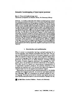
logical constraints. These optional constructions are interesting when one seeks concision. Figure 1 shows both a complete tree and the way we draw it.

ad he

sub

John

de t

⊥

⊥

walks

•. j sub

walks

obj

ad he

j

•.

Figure 1: Tree logical structure and tree drawing examples

John

To make it clear that the trees we use are just a variant of the notation of the ranked trees, we explain how to represent the trees we use as ranked trees. For this, it suffices to fix an arbitrary total order on the set of labels and to define term constructors that consist in subsets S of labels whose arity is the cardinal of S . Then the k th argument of the constructor S represents the child with the k th label in S according to the fixed order of labels. For example, fixing a total order where the label head precedes the label subj, the term representation of the tree in Figure 1 is {head, subj} walks John. Formally, given a finite set of edge labels Σ, we define a tree domain dom(t) as being a non-empty finite subset of Σ∗ , that is prefixclosed and so that if for a in Σ, ua is in dom(t), then for each b in Σ, ub is in dom(t). Given a tree domain dom(t), we write dom(t) for the set of longest strings in dom(t). The elements of dom(t) are the positions that correspond to leaves in the tree domain. Given a finite set of labels Λ, a tree t is a pair (dom(t), lbl : dom(t) → Λ ∪ {⊥}). 1 The set Λ of labels shall be the vocabulary, while Σ shall be the set of syntactic functions. Logical definition of abstract languages

We have now settled the class of objects that will serve as elements of our abstract language. We then lay out how the set of valid abstract structures is defined, that is how we specify which abstract structures are the syntactically correct ones. This process will be carried on by logic, in the sense that the set of valid abstract structures will be the set of all trees that satisfy some logical constraints. Provided that the logic expressing those constraints is 1 Of

course, we assume that ⊥ is not an element of Λ.

[ 94

]


kept simple enough, the resulting abstract language will be both suitably structured and concisely described, while being recognizable by a finite state automaton. In order to satisfy this last condition, we shall restrict our attention to the class of logical languages that only define regular tree languages. There are several reasons for this. First of all, it is easy to represent the run of a tree automaton as the abstract language of a 2-ACG, and, therefore, logical constraints that only define regular languages can be compiled as abstract languages of 2-ACGs. Second, those logics have decidable satisfiability problems and thus it is in principle possible to automatically check the coherence of a set of constraints or check whether valid abstract structures satisfy a given property. Moreover, neither of those properties are preserved in general when considering more powerful logics. Finally, it seems that linguistic constraints do not need extra logical power. The most expressive and concise logic that is known in this class is Monadic Second-Order Logic (MSOL), but various kinds of first-order or modal logics may suit very well the needs of linguistics. The logical language

We define a first-order logical language that we believe is a good candidate for describing the linguistically relevant properties of abstract structures. The set of well-formed formulae in this logic is defined in the usual way for first-order logic, with the conventional connectives (¬, ∧, ∨, ⇒, ⇔, ∃, ∀) and first-order variables ( x, y, z, . . . ) that will be interpreted as positions in the tree. Then, atomic formulae will be based on the following predicates and relations. First, we assume that we have been given a vocabulary such as the one in Table 1 that uses the finite set of properties P . Each element p of P (listed on the right in the tables representing vocabularies) will correspond to a unary predicate p(x) in our logic. By definition, such a predicate p will be true if and only if x is the position of a leaf in the tree that is labelled by a lexical entry containing p in its list of properties. From a linguistic point of view, those predicates allow us to talk about the lexical properties of words and ensure that the sentence structure is in accordance with those properties (which can be used to deal with agreement, verb valency, control, etc.).

[

95

]


Then, we add another predicate noted none(x) which is true if and only if x is a leaf labelled with ⊥. This will be particularly useful in the case of optional arguments. This predicate will enable us to condition the presence or the absence of an argument with respect to the context. We shall also write some(x) as a short-hand for ¬none(x). Since we have decided to leave the internal nodes of the tree unlabelled, no additional single-argument predicate is required. Had we chosen to add linguistic information to internal nodes, we could have introduced a set of corresponding predicates to take this information into account when defining the set of valid abstract structures. Finally, we add a countable set of binary relations that express properties about paths between nodes. This set is defined as the set of all regular expressions over the alphabet of argument labels. If we assume that the set of argument labels is Σ, then regular expressions are defined inductively with the following grammar: reg ::= ϵ | Σ | (reg + reg) | reg reg | (reg)∗

The language denoted by a regular expression is defined as usual (ϵ denoting the empty word). We shall also take the liberty of dropping useless parentheses. Let e be such a regular expression, we write L(e) for the language defined by e. Then e(x, y) is a well-formed formula that is true if and only if x is an ancestor of y and the (possibly empty) sequence of edge labels l i on the path between x and y induces a word w = l1 . . . l n such that w ∈ L(e). This set of relations could also be obtained indirectly, by using the more usual finite set of successor relations and either adding a transitive closure operator to first-order logic or using the full power of Monadic Second-Order Logic. In either case, this set of relations is intended to enable the description of longdistance phenomena in sentences (as, for example, wh-movement). In order to shorten some formulae, we also add the following relation notation: e1 ↑ e2 (x, y) which is true if and only if the lowest common ancestor z of x and y is such that e1 (z, x) and e2 (z, y). We also use the shorthand any to denote any element of Σ. Notice that the relation e1 ↑ e2 (x, y) can indeed be expressed as: ∃z.e1 (z, x) ∧ e2 (z, y) ∧ ∀z ′ . any∗ (z ′ , x) ∧ any∗ (z ′ , y) ⇒ any∗ (z ′ , z)

[ 96

]


Formally, given a tree t = (dom(t), lbl), a formula φ , and a valuation ν that maps the free variables of φ to elements of dom(t) we define the validity relation t, ν |= φ by induction on φ : 2 • t, ν |= true is always correct, • t, ν |= p(x) iff ν(x) is in dom(t) and lbl(ν(x)) = (w, Q) with p ∈ Q, • t, ν |= none(x) iff ν(x) is in dom(t) and lbl(ν(x)) = ⊥, • t, ν |= e(x, y) iff ν(x) = w1 , ν( y) = w1 w2 , and w2 ∈ L(e) for some w1 and w2 in dom(t), • t, ν |= φ ∨ ψ iff t, ν |= φ or t, ν |= ψ, • t, ν, |= ¬φ iff it is not the case that t, ν |= φ , • t, ν |= ∃x.φ iff there is u in dom(t) so that t, ν[x ← u] |= φ , where ν[x ← u] is the valuation that maps every variable y different from x to ν( y) and maps x to u. Regular over-approximation of abstract structures

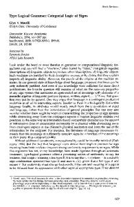
Though we believe that the class of logical formulae described above constitutes a powerful tool to describe the abstract structures of human languages, we also think that the recursive shape of these structures can be expressed by simpler and more concise means. Hence, we suggest to use regular tree grammars to provide an over-approximation of the intended abstract language, and then refine this sketch by adding logical constraints on the grammar’s productions to filter out the undesired structures. Thus, we gain the ability to model the predicateargument structure in a more readable way. In general, the regular grammar aims at modelling the recursive structure of natural languages while the constraints are meant to express relations between constituents and to ensure that these relations satisfy the grammatical constraints of the language. This over-approximation is defined by means of a regular tree grammar. Figure 2 gives such a grammar as an example. Note that some non-terminals may occur between parentheses in the right-hand sides of some rules. The intended meaning is that they are optional: given a non-terminal X , we may think of (X ) as a non-terminal that can 2 We

only treat the connectives ∃, ∨, and ¬ which are sufficient to express all the other logical connectives.

[

97

]


be rewritten to either X or ⊥. Other non-terminals are simply properties of lexical entries (one could also use sets of properties), these non-terminals may be rewritten to any lexical entry which contains this property in its list of properties. This over-approximation simply puts in place the definitions of linguistic syntagmas so as to model the hierarchical structure of language constructs. From the perspective of grammatical design, such an over-approximation should be based on high-level linguistic considerations and only take care of simple local constraints, accounting for the universals of language, or for the common features of a given family of languages. In particular, it should only use the broadest and simplest lexical properties, such as parts-of-speech.

d he a

t

noun

(A)

de

A

j

verb

p2 : A −→ •. ob

he ad

p1 : S −→ •. subj

Figure 2: Over-approximating regular tree grammar example

determiner

p3 : A −→ proper noun Constraining the regular productions

We now describe how the logical language will be used to refine the regular tree grammar productions that over-approximate the language of abstract structures. The general idea is that one or several logical formulae can be attached to each production rule of the regular grammar. For this, some nodes on the right-hand sides of rules are tagged with pairwise distinct variables (see Figure 3), and the rules are paired with a set of formulae whose free variables range over the variables that tag their right-hand sides. Now when a rule is used in the course of a derivation, the nodes it creates are constrained by the logical formula paired with the rule. Thus, once a derivation is completed, the resulting tree is considered valid only when it satisfies all the constraints that have been introduced in the course of the derivation. Let us consider Figure 3 as an example: the first production p1 of our toy grammar is now tagged with two variables respectively named

[ 98

]


he

j

ob

verb : v

subj

ad

p1 : S −→ •.

Figure 3: Labelled production rule with logical guards

(A) : o

A

some(o) ⇒ transitive(v) none(o) ⇒ intransitive(v)

v and o and which respectively designate the head and obj arguments of the root node. These labels are indicated after colons at the position that they correspond to. Below the rewrite rule is a list of logical constraints that deal with verb valency, and the logical formula φ(v, o) that the final abstract tree must satisfy is implicitly taken to be the conjunction of those two constraints. We now give a formal definition of what it means for a tree to be valid. A derivation is seen as generating a triple (t, ν, φ) where t is a tree, φ a logical formula, and ν a valuation of the free variables of φ in dom(t). The rules of the grammar act on these triples as follows: if (t, ν, φ) is such that at the position u, t has a leaf labelled with the non-terminal A and if there is a rule that rewrites A into s with the constraints φ1 (x 1 , . . . , x n ), . . . , φ p (x 1 , . . . , x n ), then (t, ν, φ) rewrites into (t ′ , ν′ , φ ∧ φ1 (x 1′ , . . . , x n′ ) ∧ · · · ∧ φ p (x 1′ , . . . , x n′ ))

where: • t ′ is obtained from t by replacing the occurrence of A at the position u by s, • x 1′ , . . . , x n′ are fresh variables, • ν′ is the valuation that maps every variable x distinct from the x i′ ’s to ν(x) and that maps each variable x i′ , to uui when ui is the position of the node that is tagged with x i in s. Now, a tree t that does not contain any occurrence of a non-terminal is valid when, with ; being the empty valuation and S being the starting symbol of the regular grammar, (S, ;, true) rewrites (in any number of steps) to (t, ν, φ), so that t, ν |= φ . We shall call language or set of valid

[

99

]


trees the set of trees that are generated by the regular grammar and satisfy the logical constraints. Compilation of logical constraints

We are going to show here that the set of valid trees, i.e. the trees generated by the regular grammar that satisfy the logical constraints, is also a regular set. Actually, since we restricted ourselves to a logical language weaker than MSOL, the constraints can be seen as a sort of regular “look-around” for the regular grammar which explains why the valid trees form a regular language. We outline here a construction that defines effectively the language of valid trees as a regular language. This construction is going to be at a rather high-level and is mainly meant to convince the reader that the set of valid trees is indeed regular. In order to simplify the construction, we first transform the set of constraints associated with rules that bear on several nodes in the right-hand side of a rule into a unique constraint that bears on the root node of the right-hand side. For this, if φ1 (x 1 , . . . , x n ), . . . , φ p (x 1 , . . . , x n ) is the set of constraints that are associated with a production r , then there is a unique path labelled with the word ei that leads from the root of the tree in the right-hand side of r to the node labelled x i , and then, for the nodes labelled x 1 , . . . , x n , to satisfy the constraints φ1 (x 1 , . . . , x n ), . . . , φ p (x 1 , . . . , x n ) is equivalent to the root satisfying the unique constraint: ψ r (x) = ∃x 1 , . . . , x n .e1 (x, x 1 ) ∧ · · · ∧ en (x, x n ) ∧

p ∧

φi (x 1 . . . , x n )

i=1

Thus, for the construction we are going to present, we assume that each rule has a unique constraint that bears on the root of its right-hand side. Given such a grammar G , we first remark that the set F of constraints used in rules is finite. We then construct a grammar G ′ so that each node of G ′ is labelled with the set of constraints included in F that it needs to satisfy. Hence, in the trees generated by G ′ , sets of formulae are labels of internal nodes. We extend our logical language with predicates that reify those labels. Thus, given a set of formulae S included in F we define a unary predicate [S](x) that holds true on nodes x that are labelled with S . The predicates used to define the constraint language keep

[ 100

]


their former meaning. We can now define a formula valid as follows: ∧

valid ::=

∀x.[S](x) ⇒

S ⊆ F

∧

φ(x)

φ(x) ∈ S

As valid is a constraint that is definable in the logical language we have introduced which in turn can be represented in Monadic Second-Order Logic, the set of trees that satisfy this constraint is regular. Thus, the set V of trees generated by G ′ that satisfy valid, being the intersection of two regular sets, is also regular. Now, the set of valid trees of G is precisely the set of trees in V where the labels of internal nodes have been erased. As regular languages are closed under relabelling, this explains why the set of valid trees is regular. Let us now briefly sketch how G ′ is constructed. Its non-terminals are pairs (A, S) so that A is a non-terminal of G and S is included in F . Each rule r of G of the form A → t with constraint φ(x) on its root is mapped to a rule (A, S) → t ′ of G ′ so that if t is reduced to a non-terminal B , then t ′ is (B, S ∪ {φ(x)}); if t is not reduced to a nonterminal, then t ′ is the tree t where the occurrences of non-terminals B of G are replaced by the non-terminals (B, ;) of G ′ and the root of t ′ is labelled with the set of formulae S ∪ {φ(x)}. This transformation is illustrated in Figure 4.

l1

lb

lb

−→

(B1 , ;)

...

ln lb

Bn

...

ln

...

Figure 4: Transformation of a rule in G into rules of G ′

. r ′ : (A, S) −→ S ∪ {φ(x)} lb

B1

...

l1

r : A −→ •. : x

(Bn , ;)

φ(x)

2.2

The linearization process

We are now going to explain how we intend to linearize the accepted sentences, by describing mappings from the set of valid abstract structures to various languages of surface realizations, which may either

[

101

]


represent the actual sequence of words, or the semantic interpretation of the sentence, or any other structure of interest. Since we have elected to work within the framework of second order ACGs, linearizations can be seen as high-level specifications of lexicons (in the sense of abstract categorial grammars), that is to say morphisms from the trees that belong to the abstract language to simply typed λ-terms of a specific object language. The signature upon which we build the simply typed λ-terms of the object language may vary, but we give here some straightforward examples of target languages for our toy grammar. We assume that the reader is familiar with simply typed λ-calculus (see Hindley and Seldin (2008) and Barendregt (1984) for more details), and contrary to what is usual in ACG, we also use product types, that is the ability to use typed pairs and the related projections in the calculus. It is well-known that this does not increase the expressive power of ACGs, but these constructs are often convenient and intuitive. Surface structures

V

L

When mapping abstract structures to surface structures of a language (English, German, and Dutch in this paper), we assume that we can freely handle sequences of words within simply typed λ-calculus (a canonical encoding of those sequences is given by de Groote (2001)). When dealing with mapping abstract structures to meaning representations, we build an appropriate signature for Montague-style semantics with atomic types that denote propositions ( p) and entities (e) and a set of constants that include the usual logical connectives ( p→p , p→p→p , E(e→p)→p , etc.). We add additional constants for verb predicates (walkse→p , lovese→e→p ) and actual entities (Johne , Marye ). Notice that to avoid confusion between the logical formula we use for syntax from the logical formula representing truth-conditions in Montague semantics, we use a different font for the connectives of the two logical languages. There are many other choices of signatures and constants for semantic representation, depending on which theory of semantic representation one adheres to. Nevertheless, any set of formulae that can be adequately represented by terms of a 2-ACG’s object language may be used for semantic representation in this formalism.

[ 102

]

A logical approach to grammar description The linearization process

The mapping between abstract structures and surface structures is defined by associating linearization rules with the production rules of the regular grammar. This mapping is mediated by the analyses of abstract structures by the regular grammar. Realizations are indeed associated to parse trees of abstract structures in the regular grammar. Nevertheless, as we wish to guide the way realizations are computed with logical constraints over abstract structures, we need to relate nodes of parse trees to nodes in abstract structures. This relation is as follows: each node in the parse tree corresponds to the use of a rule. Such a rule rewrites a non-terminal to a tree that occurs in the abstract structure. As a convention, we associate the root of that tree with the node in the parse tree. Notice that due to possible ε-rules in the regular grammar, i.e. rules of the form A → B , where B is another non-terminal, there may be several nodes in the parse trees that are related to the same node in the abstract structure; there may also be nodes in the abstract structure that are not related to any node in the parse tree by our convention. This is simply because they are inner nodes of some right-hand side of a rule. Observe also that when a node in the abstract structure is related to several nodes in the parse tree, all those nodes form a chain in the parse tree (all of them correspond to an ε-rule) and they are thus totally ordered. Since, once we have fixed a parse tree, it is convenient to associate realizations with nodes in the abstract structure, we take the convention that the realization of a node x ′ in the abstract structure is the realization of the node x at the highest position in the parse structure that is related to x ′ . The realization of nodes in the parse tree may depend on several parameters: (i) the realization of the other non-terminals that occur in the right-hand side of the production, (ii) the context in which the rule is used (for example the realization of German or Dutch subordinate clauses differ from that of the main clause), (iii) the realization of nodes that appear elsewhere in the abstract structure, typically, this shall be the case in the presence of wh-movement. In order to take all those constraints into account, given a rule A → t of the regular grammar, we tag the non-terminal A with a variable x 0 and assume that the non-terminals that occur in t are labelled with

[

103

]


the variables x 1 , …, x n . Then the linearization rules are expressed as a list of the form: real(x 0 ) ::= φ(x 0 , x 1 , . . . , x n , y1 , . . . , ym ) → M [real(x 1 ), . . . , real(x n ), real( y1 ), . . . , real( ym )]

where M is a simply typed λ-term that is meant to combine the realizations of the nodes denoted by x 0 , …, x n , y1 , …, ym . The variables y1 , . . . , ym are not tagging any node in the right-hand side of the rule. The variables y1 , . . . , ym represent nodes of a complete abstract structure (i.e. nodes from the context in which the rule is used), which makes the formula φ(x 0 , x 1 , . . . , x n , y1 , . . . , ym ) true in the abstract structure (here x 0 is interpreted as the node in the abstract tree that is related to the use of the rule, i.e., by our convention, the root of the subtree generated by the rule). In linearization rules, we shall call internal variables those variables (the x i ’s) that are tagging the production rules, while we shall call the other (the yi ’s) external variables. The intended meaning of such a rule is that given nodes y1 , . . . , ym in the abstract structure so that φ(x 0 , x 1 , . . . , x n , y1 , . . . , ym ) holds true, if the realizations of x 1 , . . . , x n , y1 , . . . , ym respectively are real(x 1 ), . . . , real(x n ), real( y1 ), . . . , real( ym ) then the realization real(x 0 ) of x 0 is the (simply typed) λ-term M [real(x 1 ), . . . , real(x n ), real( y1 ), . . . , real( ym )] .

The realization of lexical entries needs to be explicitly given. For the particular case of phonological realizations, we assume that each lexical entry is realized as the very word given by the entry. Then a realization of a parse tree is a realization of its root. By extension, a realization of an abstract structure is a realization of one of its parse trees. Importantly, two different linearization rules need not use λterms that have the same type. Indeed, depending on the context, a rule may give rise to realizations that have distinct types. An example of this is provided by the realizations of Dutch clauses depending on whether they are relative clauses or main clauses: in the case of main clauses, the realization is simply a string, while in the case of relative clauses, the realization is a pair of strings so as to compute the cross serial placement of arguments and verbs (see Section 3.1). The use of external variables is motivated by the linguistic notion of movement in syntax. Indeed, we shall see in Section 3 how to move

[ 104

]


a relative pronoun from its canonical place in the abstract structure to its landing site in front of the linearization of a relative clause. A priori, linearization rules associate non-deterministically a set of realizations with a given parse tree of an abstract structure. Indeed, there are two sources of non-determinism: (i) there may be several linearization rules that may apply in a given node of the parse tree, (ii) there may be several tuples y1 , . . . , ym that make the formula φ(x 0 , x 1 , . . . , x n , y1 , . . . , ym ) true. The use of non-determinism may be of interest for linguistic models where some surface variation has no incidence on the syntactic relations between the constituents like for example the order of circumstantial clauses in French.

he

j

c :=

(A) : o

A:s

transitive(v) intransitive(v)

Figure 5: Example of a guided linearization

ob

verb : v

subj

ad

S : c −→ •.

−→ −→

svo sv

Figure 5 gives an example of a linearization rule. This rule, as most of the rules we shall meet later, does not use external variables. To make the writing of rules shorter, we shall write realizations in the teletype font, that is, v, s, o instead of real(v), real(s), real(o). It is worthwhile to notice that the presence of external variables can be problematic for realizations. Indeed, using this mechanism, it is not hard to realize two nodes x and y so that the realization of x depends on that of y and vice versa. In such a case we assume that the realization is ill-formed and do not consider it. In the linguistic examples we have considered so far, this situation has never arisen as the external variables y1 , . . . , ym on which the realization of a node x depends are always strictly dominated by that node x . Nevertheless, from a theoretical point of view, we show in the discussion at the end of the section that the situations giving rise to circular definitions can be filtered out with usual finite state automata techniques. We now give a formal definition of what it means for an abstract structure t to be realized by a term M . For the sake of simplicity and without loss of generality (as we have seen in Section 2.1, page 100),

[

105

]


we assume that the grammars we use have constraints that bear only on the root of the right-hand sides of rules. Thus, given a constrained grammar with linearization rules, such a grammar generates 5-tuples (E, V, t, ν, φ) where: • t is a tree, • φ is a logical formula, • ν is a valuation of some of the free variables of φ in dom(t), • V is a function from the positions of t which are labelled with non-terminals to variables that are free in φ , • E is a deterministic grammar (i.e. each of its non-terminals can be rewritten with at most one rule) whose non-terminals are the free variables in φ ; the rules of the grammar rewrite non-terminals to λ-terms (that may contain occurrences of non-terminals). Moreover, the variables occurring in the right-hand sides of rules but not in the left-hand sides are either variables that are mapped to a position of a non-terminal in t by V , or which are not in the domain of ν (i.e. external variables). As we have defined valid abstract structures, t is the abstract structure being produced, φ is a logical formula that the completely derived tree needs to verify. The valuation ν is a bit different from the definition of valid abstract structures in that it does not map every variable that is free in φ to a node in t . This is due to the external variables that need to be found once the derivation is completed. The other elements of the tuple, namely E and V , are there to construct a parse tree and maintain the relation between the nodes of the parse tree and the nodes of t , respecting the convention we spelled out earlier. The unique derivation of E actually represents the parse tree being constructed, while its rewriting rules contain the necessary information to construct the realization. The function V maps the nonterminals occurring in t to variables that shall later be used in the construction of E once they are rewritten. The relation between the nodes in the parse tree and the nodes in the abstract tree is maintained by ν via the use of variables: a variable x that is a non-terminal in E represents the use of a rule (i.e. a node in the parse tree) which is related to the node ν(x) of t . The role of V is to permit the extension of the relation in the course of the derivation.

[ 106

]


Let us now see how this works. A rule of the grammar such as the one given in Figure 6 can act on such a tuple. Let us consider a tree t that has an occurrence of the non-terminal A at position u. Then a rule of the form A → s can rewrite a tuple (E, V, t, ν, φ) into ′ (E ′ , V ′ , t ′ , ν′ , φ ∧ ψ(x 0′ ) ∧ ψk (x 0′ , . . . , x n′ , y1′ , . . . , ym ))

where: • t ′ is obtained from t by replacing the occurrence of A at position u by s, • x 0′ = V (u), • x 1′ , …, x n′ , y1′ , …, ym′ are fresh variables, • ν′ is the valuation that maps every variable x distinct from the x i′ ’s (i ̸= 0) and the y ′j ’s to ν(x) and that maps each variable x i′ , with 1 ≤ i ≤ n, to ul i when l i is the position of the node that is tagged with x i in s, • 1 ≤ k ≤ p, is the index of the possible realization chosen for the rule; it corresponds to the choice of a formula ψk (x 0 . . . x n , y1 . . . ym ) and the corresponding realization Mk , • V ′ is equal to V for positions different from ul1 , …, ul n and V ′ (ul i ) = x i′ for 1 ≤ i ≤ n, • E ′ is E to which we add the rule x 0′ → Mk′ and where Mk′ is obtained from Mk by respectively substituting x 1′ , …, x n′ , y1′ , …, ym′ for x 1 , …, x n , y1 , …, ym . A −→

A1 : x 1

...

l1

• : .x 0

Figure 6: Constrained production with its associated linearization rule

ln

...

An : x n

ψ(x 0 . . . x n ) ψ1 (x 0 . . . x n , y1 . . . ym ) −→ M1 .. .. .. x0 := . . . ψ p (x 0 . . . x n , y1 . . . ym ) −→ Mp (Where the free variables in M1 . . . Mp are x1 . . . xn y1 . . . ym .)

[

107

]


A rule A → w that rewrites a non-terminal into a lexical entry w, assuming that this lexical entry is associated with the realization w, can rewrite (E, V, t, ν, φ) into (E ′ , V, t ′ , ν, φ) where: • t ′ is obtained by replacing the occurrence of the non-terminal A at the position u by w, • E ′ is the grammar obtained from E by adding the rule x → w if V (u) = x . A complete derivation is a derivation such that (;, (ϵ, x), S, ;, true) rewrites in several steps into (E, V, t, ν, φ), where t does not contain any occurrence of a non-terminal. The rules of E define a unique term, but this term may be not well-typed, or it may contain some free variables due to the external variables of some rule used in the course of the derivation. In the first case, we consider the derivation as invalid, in the second case, we need to give a meaning to the free variables of the term defined by E . For this, we need a valuation ν′ that extends ν by mapping the free variables of φ for which ν is undefined to ν(dom(E)), where dom(E) is the set of variables that are non-terminals of E . Thus ν′ extends ν by mapping the external variables to nodes of t which are related to some node in the parse tree implicitly represented by E . Moreover, ν′ need to be such that t, ν′ |= φ . Notice that, in particular, this forces t to be a valid tree of the underlying regular grammar of abstract structures, as φ contains as one of its conjuncts the formula that t should satisfy in order to be valid. Now that ν′ is given, we may assign a semantics to the free variables in the term defined by E . For this, we follow our convention, by associating with an external variable y the realization of the node ν( y). Technically, it suffices to remark that, as E is a deterministic grammar, its rules induce a partial order on the non-terminals of E . Using this partial order, we replace each occurrence of a parameter y by the maximal non-terminal x in E so that ν′ (x) = ν′ ( y). If we do this for each parameter y , we obtain a deterministic grammar E ′ ; if this grammar defines a finite well-typed term, this term must be unique and we call it realization of (E, V, t, ν, φ). Nevertheless, E ′ may not define any finite term due to circular definitions, and it may also define badly typed terms. Thus, in a nutshell, given the result (E, V, t, ν, φ) of a complete derivation, its set of realizations M is given by every extension ν′ so that

[ 108

]


t, ν′ |= φ , so that the grammar E ′ that ν′ induces defines the well-typed term M ′ , whose normal form is M . Notice that, with this definition, a non-valid tree has an empty set of realizations. More abstractly, we may see the linearization process as a Monadic Second-Order transduction (MSO-transduction) in the sense of Courcelle (1994) that turns the parse tree of a valid tree into a Directed Acyclic Graph (DAG) whose nodes are labelled with λ-terms. Then we take the unfolding of this DAG into a tree which can then be seen as a λ-term. The final step consists in β -normalizing this term provided it is well-typed. Courcelle and Engelfriet (1995) (see also Courcelle and Engelfriet 2012 for a more recent presentation of that result) showed that the class of languages definable with Hyperedge Replacement Grammars (HRG) is closed under MSO-transductions. As regular languages can easily be represented as HRGs, this shows that the language of DAGs output by the linearization process is definable by a Hyperedge Replacement Grammar (HRGs). Moreover, as shown by Engelfriet and Heyker (1992), the tree languages that are unfoldings of DAG languages definable with HRGs are output languages of attribute grammars, which in turn can be seen as almost linear 2-ACGs as showed by Kanazawa (2011, 2009). Thus, taking another homomorphism yields in general a non-linear 2-ACG. Nevertheless, when modelling the phonological realizations, we expect that the language we obtain is a linear 2-ACG. It is worthwhile to notice that the acyclicity of a graph is a definable property in MSO, and also that the well-typing of a tree labelled by λ-terms is MSO definable as well. Moreover, the translation of the linearization rules into a 2-ACG is such that the abstract syntactic structure can be read from the derivation trees of the 2-ACG we obtain with a simple relabelling. Indeed, when we showed how to construct a regular grammar recognizing the set of valid abstract structures, the abstract language of the 2-ACG was obtained by enriching the derivation trees of the regular grammar with information about the states of the automata corresponding to the logical formula or to the typing constraints. Therefore, the regular grammar with constraints and linearization rules can be effectively compiled into a 2-ACG. It is worthwhile to notice that the compiled grammar may be much larger than the original description.

[

109

]

Lionel Clément et al. Handling optional arguments

We have proposed earlier to use (A) in regular tree productions to denote that an argument A is optional. Such an optional argument is then taken as a non-terminal that can rewrite into either A or ⊥. When defining a linearization, the realization of (A) is taken to be that of the symbol that it rewrites to. We will set some default value as the realization of ⊥, so that the realization of an empty argument is well defined. For instance, in the example described by Figure 5, a sensible value for ⊥ is the empty string ϵ . With this default value, we may simply have one linearization rule c := true −→ s v o. Thus, when the verb is intransitive, the constraints we have put on the valid trees imply that the obj argument in the tree must be ⊥. Taking the empty string as a default value, we get s v o = s v, which is the expected realization of an intransitive verb clause. We can choose to provide each optional argument with its own default values, depending on what we consider a sensible realization of an empty optional argument. We could also conceivably associate a value with ⊥ that depends on its context in a stronger way, by using logical formulae. However, we have not found it useful in the models we have worked on; therefore, the linearization of optional arguments will only be ϵ for phonological linearizations, and a semantically empty argument when linearizing towards a sentence meaning representation. Additional macro syntax

The main goal of our approach is concision. To avoid redundancy in linearization rules, we introduce a syntactic mechanism that factors out some redundant constructions. Indeed, the number of linearization rules depend on the number of syntactic situations that may have an influence on the form the linearization takes. This number can be rather high, and just listing the situations may give the impression that one misses obvious generalizations, or structural dependencies between various cases. The mechanism we propose to cope with this problem tries to give more structure to linearization rules. Mainly this mechanism is a form of simply typed λ-calculus designed to manipulate the linearization

[ 110

]


rules. This calculus is parametrized with a finite set of variables X of the syntactic logical language. We write F O[X ] as a shorthand for the set of logical formulae whose set of free variables is included in X . The set of types of the language is divided into two disjoint sets: otypes and ωtypes. The set otypes is the set of simple types of the object language (i.e. the target language of the linearization) and ωtypes are types of the form A1 → · · · → An → ω, where ω is an atomic type that is distinct from the atomic types used in otypes and A1 , …, An are otypes. As we have seen, one of the features of the linearization mechanism is that, depending on the context, the type of the realization may vary. Thus, in general, linearization rules are objects of the form [φ1 −→ M1 , . . . , φn −→ Mn ], where M1 , . . . , Mn are terms that may have different types. The atomic type ω is meant to type these objects. The set of terms of the language, TA,X , is thus indexed with two parameters: A is either an otypes or an ωtypes and X is the set of variables that are allowed to be free in the logical formula. The sets TA,X are inductively defined as follows: • for A in otypes, x A is in TA,X , • if M and N are respectively in TA→B,X and in TA,X , then M N is in TB,X , • if M is in TB,X and A is in otypes then λx A.M is in TA→B,X , • if M1 , . . . , Mn are all in TA,X with A in otypes and φ1 , . . . , φn are all in F O[X ], then [φ1 −→ M1 , · · · φn −→ Mn ] is in TA,X , • if M1 , . . . , Mn are respectively in TA1 ,X , . . . , TAn ,X with the A1 , . . . , An either being equal to ω or being in otypes, then and φ1 , . . . , φn are all in F O[X ], then [φ1 −→ M1 , · · · , φn −→ Mn ] is in Tω,X . We adopt a call-by-value operational semantics for this language: as for IO languages (see Kobele and Salvati 2013), the notion of value coincides with that of the normal form. For this we need the notion of pure terms, that is λ-terms which contain no construct of the form [φ1 −→ M1 , · · · , φn −→ Mn ]. We shall denote pure terms in β -normal form with V , possibly with indices. A term is said to be in the normal form either when it is a pure term in the β -normal form, or when it is a term of the form [φ1 −→ M1 , . . . , φn −→ Mn ], where M1 , . . . , Mn are pure terms in the β -normal form. From now on we shall write W , possibly with indices, for terms that are values, that is terms in normal

[

111

]


form. The computational rules of the calculus are as follows ( M [V /x] denotes the capture-avoiding substitution of V for the free occurrences of x in M ): • (λx.M )V → M [V /x], • (λx.M )[φ1 −→ V1 , . . . , φn −→ Vn ] → [φ1 −→ M [V1 /x], . . . , φn −→ M [Vn /x]], • [φ1 −→ M1 , . . . , φn −→ Mn ]W → [φ1 −→ M1 W, . . . , φn −→ Mn W ], • λx.[φ1 −→ V1 , . . . , φn −→ Vn ] → [φ1 −→ λx.V1 , . . . , φn −→ λx.Vn ], • V [φ1 −→ V1 , . . . , φn −→ Vn ] → [φ1 −→ V V1 , . . . , φn −→ V Vn ] when V is not a λ-abstraction, • [φ1 −→ M1 , . . . , φk −→ [ψ1 −→ V1 , . . . , ψn −→ Vn ], . . . , φm −→ Mm ] → [φ1 −→ M1 , . . . , φk ∧ ψ1 −→ V1 , . . . , φk ∧ ψn −→ Vn , . . . , φm −→ Mm ]. The strong normalization of the simply typed λ-calculus induces the fact that computations in that calculus are terminating. The subject reduction property (the fact that the types of terms are invariant under reduction) is also inherited from the simply typed λ-calculus. We adopt in general a right-most reduction strategy which consists in rewriting the redex that is at the furthest right position in the term. This implements a call-by-value semantics for this language. Finally, in the rest of the paper, we shall adopt some slight variation on the syntax of the language. In particular, we shall omit the typing annotations most of the time. We shall also write structures like [φ1 −→ M1 , . . . , φn −→ Mn ] as column vectors in which we omit the ’,’ comma separator. We may also omit the square brackets or only put the left one to lighten the notation. We may write M where x 1 = M1 and . . . and x n = Mn in place of (λx 1 . . . x n .M )M1 . . . Mn . Another abbreviation consists in simply writing M for [true −→ M ]. Finally when we write [φ1 −→ M1 , . . . , φn −→ Mn , else −→ M ] we mean [φ1 −→ M1 , . . . , φn −→ Mn , ¬φ1 ∧ · · · ∧ ¬φn −→ M ]. Examples of this notation are used all along the next section.

[ 112

]

A logical approach to grammar description 3 3.1

illustration Synchronous grammar

We now illustrate the formalism we have introduced in the previous section by constructing a more complex grammar. This grammar will provide a superficial cover of several overlapping phenomena. It covers verbal clauses with subject, direct object, and complement clause arguments, taking into account verb valency. It also includes subject and object control verbs, and modification of noun phrases by relative clauses, with a wh-movement account of relative pronouns that takes island constraints into account. It also models a simplistic case of agreement that only restricts the use of the relative pronoun that to neuter antecedent. Linearization rules are provided that produce phonological realizations for English, German, and Dutch, in order to demonstrate the possibility of parametrizing the word order of realizations (including cross-serial ordering). Another set of linearization rules produces Montague-style λ-terms that represent the meaning of the covered sentences. Even though we have chosen our example so as to avoid a complete coverage of agreement, we hope that the treatment of that is illustrative enough to give a flavor of its rather straightforward extension to a realistic model of agreement. Our goal when designing this grammar is to confront the methodology described so far against the task of dealing with the modeling of several interacting phenomena, along with both their syntactic and semantic linearizations, and evaluate the results in terms of expressiveness as well as concision. Vocabulary

First, we construct a vocabulary for our grammar. The part-of-speech properties we use are: proper_noun, noun, pronoun, determiner, verb. The other lexical properties are: pro_rel, transitive, ctr_subj, ctr_obj, infinitive, masculine, feminine, neuter and designate respectively: relative pronouns, transitive verbs, subject control, and object control verbs, verbs in infinitive form, and gender marking.

[

113

]

Lionel Clément et al. Table 2: Excerpt vocabulary

English German Dutch Semantic type Properties lets

lässt

help

helpen

helfen e → e → p → p verb; ctr_obj; transitive; infinitive

laat

e → e → p → p verb; ctr_obj; transitive

want

willen

wilen

e→p→p

verb; ctr_subj; infinitive

read

lesen

lezen

e→e→p

verb; transitive; infinitive

that

das

dat

(e → p) → p

pronoun; pro_rel; neuter

a

ein

een

(e → p) → p

determiner; neuter

book

Buch

boek

e→p

noun; neuter

John

Hans

Jan

e

proper_noun; masculine

Mary

Marie

Marie

e

proper_noun; feminine

Ann

Anna

Anna

e

proper_noun; feminine

The vocabulary is summed up in Table 2. The table also gives the expected phonological realizations of the individual lexical entries for English, German, and Dutch, along with the type of their semantic realization. Semantic types are based on e and p, which denote entities and propositions (truth values), respectively. Abstract structure leaves that are lexical entries will be written as their associated English realizations; and so will their semantic realizations, with the same typesetting conventions we used previously: e.g. song (abstract structure leaf) vs. song (semantic realization). Regular over-approximation

We now present the regular grammar that over-approximates the set of valid abstract structures. It contains three non-terminal symbols C , A, and M . The start symbol C corresponds to independent or subordinate clauses, A to noun phrases that are an argument of some clause, and M to modifiers. The labels used on the edges of abstract structures belong to the list (head, subj, obj, arg_cl, det, mod) and designate respectively the head of the (nominal or verbal) phrase, the nominal subject, the nominal direct object, an additional complement clause of the verbal predicate, the determiner in a noun phrase, and a modifier. The production rules of the grammar are given in Figure 7. The production p1 constructs a clause with a verb as its head, along with its (optional) arguments; p2 recursively adds a modifier to an argument; p3 through p5 build an argument as a noun phrase, respectively in the

[ 114

]


p1 : C −→ •. : t j

sub

verb : v

(A) : s

(A) : o

cl (C) : c

p4 : A −→ proper_noun : pn

noun : n

t

M:m

de

mo

A: a

d

he a

p3 : A −→•. he ad

p2 : A −→•. d

ar g_

obj

ad he

determiner : d

p5 : A −→ pronoun : p

p6 : M −→ C : r

form of a determiner/noun pair, a proper noun, and a pronoun; and finally p6 constructs a modifier as a verbal clause. Note that the only type of modifiers covered in the grammar are verbal clauses (which we shall restrict to be relative clauses), but other could be added by adding more productions that rewrite M as an adjective or a genitive construct. Defining linguistic notions

We now use the logical language to construct predicates that model linguistic notions and relations. We shall use these relations both for constraining the regular grammar and to guide the linearization process. The predicates and relations we add are summed up in Table 3. The first predicate recognizes a control verb which is simply a verb that has the subject control or object control lexical property: control_verb(v) := verb(v) ∧ (ctr_subj(v) ∨ ctr_obj(v)) The second predicate defines a clause as a subtree whose head is a verb: clause(cl) := ∃v.verb(v) ∧ head(cl, v) Then, a controlled clause is a clause that serves as an argument of a control verb: controlled(ctd) := clause(ctd) ∧ ∃ctr.control_verb(ctr) ∧ head ↑ arg_cl(ctr, ctd)

We construct another predicate to identify verbs that expect an argument clause. In the context of our grammar, this is equivalent to

[

115

]

Figure 7: Regular overapproximation of valid sentences

Lionel Clément et al. Table 3: Logical predicates modelling linguistic notions

control_verb(v) := verb(v) ∧ (ctr_subj(v) ∨ ctr_obj(v)) clause(vp) := ∃v.verb(v) ∧ head(vp, v) controlled(ctd) := clause(ctd) ∧ ∃ctr.control_verb(ctr) ∧ head ↑ arg_cl(ctr, ctd) clause_verb(v) := control_verb(v) independent(icl) := clause(icl) ∧ ∀cl.clause(cl) ⇒ ¬any+ (cl, icl) subordinate(scl) := clause(scl) ∧ ∃p.(mod + arg_cl)(p, scl) relative(rcl) := subordinate(rcl) ∧ ∃hd.(noun(hd) ∨ proper_noun(hd)) ∧ head∗ ↑ mod(hd, rcl)

ext_path(cl, p) := (subj + arg_cl∗ obj)(cl, p) ext_obj(obj) := pro_rel(obj) ∧ ∃cl.obj(cl, obj) ext_suj(suj) := pro_rel(suj) ∧ ∃cl.subj(cl, suj) ext_cl(cl) := ∃p.ext_path(cl, p) ∧ pro_rel(p) gd_agr(x, y) := (masculine(x) ∧ masculine( y)) ∨ (feminine(x) ∧ feminine( y)) ∨ (neuter(x) ∧ neuter( y))

antecedent(ant, pro) := (noun(ant) ∨ proper_noun(ant)) ∧ pro_rel(pro) ∧ ∃rcl.relative(rcl) ∧ head∗ ↑ mod(ant, rcl) ∧ ext_path(rcl, pro)

the verb being a (subject or object) control verb: clause_verb(v) := control_verb(v) This predicate could be extended to include verbs that expect other forms of complement clauses besides the infinitival clauses associated with control verbs. The following predicates enable us to distinguish between different types of clauses. First, an independent clause is a clause that is not dominated (through any non-empty sequence of edges) by any other clause: independent(icl) := clause(icl) ∧ ∀cl.clause(cl) ⇒ ¬any+ (cl, icl) By contrast, a subordinate clause is a clause that serves as a complement or modifier: subordinate(scl) := clause(scl) ∧ ∃p.(mod + arg_cl)(p, scl)

[ 116

]


Then, a relative clause is a subordinate clause that modifies a noun phrase (a subtree whose head is a common or proper noun): relative(rcl) := subordinate(rcl) ∧ ∃hd.(noun(hd) ∨ proper_noun(hd)) ∧ head∗ ↑ mod(hd, rcl) We then add a predicate to identify objects that undergo a whmovement (which we call extracted). This covers all relative pronouns that fill an object role in a clause. We also provide a similar predicate for extracted subjects, following the usual analysis of generative grammars (Chomsky 1981): ext_obj(obj) := pro_rel(obj) ∧ ∃cl.obj(cl, obj) ext_suj(suj) := pro_rel(suj) ∧ ∃cl.subj(cl, suj) Next, we add a relation that links an insertion site and its corresponding extraction site, taking into account island constraints as defined by Ross (1967). We recall that, in the generative tradition, the extraction site is the position at which a wh-word would be realized given its syntactic role according to the canonical word order of a language. By contrast, the insertion site corresponds to its actual position in the sentence. In our grammar, complying with island constraints means that only arg_cl edges are allowed for traversal before we reach a distant extracted object: ext_path(cl, p) := (subj + arg_cl∗ obj)(cl, p) Using this relation, we define another predicate, which denotes that a complement clause contains an extraction of some form; this corresponds to the clause containing a relative pronoun at the end of a valid extraction path: ext_cl(cl) := ∃p.ext_path(cl, p) ∧ pro_rel(p) Note that the straightforward definition of ext_path we have given does not, purposefully, guarantee that the first position given is an insertion site, nor that the second one is an extraction site. It simply ensures that island constraints are not violated for long-distance extractions in the context of our grammar. However, since we are only going to use

[

117

]


it in contexts where both its arguments must satisfy the other prerequisites for wh-movement, this simple definition will be sufficient for our needs. We add another relation that verifies gender agreement between two nodes. This relation is simply true if and only if both of the involved nodes have the same gender property: gd_agr(x, y) := masculine(x) ∧ masculine( y) ∨ feminine(x) ∧ feminine( y) ∨ neuter(x) ∧ neuter( y) This relation could be extended so as to account for more agreement phenomena such as number, case, etc. Finally, we define one last relation that links a relative pronoun to its antecedent. This relation is built upon ext_path and links the head of a noun phrase to the relative pronoun of the relative clause that modifies it: antecedent(ant, pro) := (noun(ant) ∨ proper_noun(ant)) ∧ pro_rel(pro) ∧ ∃rcl.relative(rcl) ∧ head∗ ↑ mod(ant, rcl) ∧ ext_path(rcl, pro) This relation will allow us to verify that relative pronouns agree with their antecedents. Logical constraints

In order to refine the over-approximation given in Figure 7, we now add logical constraints to production rules. We recall that only the abstract structures which satisfy these formulae are considered valid according to the grammar, thus filtering out many ill-formed structures. We first consider p1 , for which four additional constraints are given in Figure 8. Constraints (1) and (2) deal with verb valency, ensuring that the produced clause has an object if and only if the head is a transitive verb, and a complement clause if and only if the head is a verb that expects one. Constraint (3) equates the lack of an explicit subject argument with the fact that a clause is controlled. From a syntactic point of view, our model uses clauses without an explicit subject. We shall see later how logic allows us to associate its subject with a controlled clause. Finally, constraint (4) ensures that verbs in controlled clauses

[ 118

]


C −→ •. : t ar

d sub j

verb : v

obj

a he

(A) : s

(A) : o

g_c

Figure 8: Logical constraints for p1

l (C) : c

transitive(v) ⇔ some(o)

(1)

clause_verb(v) ⇔ some(c)

(2)

controlled(t) ⇔ none(s)

(3)

controlled(t) ⇔ infinitive(v)

(4)

are in an infinitive form and, since the grammar does not handle other kinds of infinitive clauses, we assume that all infinitive verbs are controlled. We now consider the relation between relative clauses and relative pronouns. We want to ensure that the valid abstract structures show a one-to-one relation between relative pronouns and the relative clauses they belong to. These pronouns should also be found at positions in their relative clause that are consistent with island constraints. This is guaranteed by a pair of symmetrical constraints on productions p5 and p6 : p5 : A −→ pronoun : p

p6 : M −→ C : r

pro_rel(p) ⇒ ∃!r.relative(r) ∧ ext_path(r, p)

∃!p.pro_rel(p) ∧ ext_path(r, p)

pro_rel(p) ⇒ ∃ant.antecedent(ant, p) ∧ gd_agr(ant, p) The production p5 rewrites an argument A as a pronoun. The first constraint associated with it ensures that, if it is a relative pronoun, there is a unique relative clause to which this pronoun corresponds. Conversely, p6 produces a relative clause and ensures that there is a unique relative pronoun that corresponds to it. Both constraints use the ext_path relation to make sure that the path between the top of the relative clause and its corresponding pronoun is valid and does not violate island constraints.

[

119

]


Then, the second constraint on p5 ensures that a relative pronoun has an antecedent, and that both of them are in agreement. With this, we rule out constructs like “Mary that …” in English, “Marie das …” in German or “Marie dat …” in Dutch. This illustrates how agreement can be added to the grammar. However, as languages may have different sets of gender and agreement rules, when dealing with synchronous grammars, it is better to model agreement by refining a core common grammar for each target language. We here avoid this complication for the sake of keeping the illustration of the formalism rather simple. This is why we only give a simplistic treatment of the neuter gender that behaves similarly in English, Dutch, and German for the particular set of sentences we model. Finally, one last syntactic restriction that we want to add is to forbid the addition of a modifier to a relative pronoun (which would be ungrammatical). The corresponding constraint is added to p2 as shown in Figure 9.

A: a

M :m

d

he ad

A −→ •. mo

Figure 9: Logical constraint of p2

¬pro_rel(a)

The added logical constraint simply ensures that a modified argument a cannot be a relative pronoun. Phonological linearizations

Finally, we turn to the process of describing four linearizations (towards English, German and Dutch on one hand, and semantics on the other hand) of the grammar. We will begin with the phonological linearizations, starting with the most straightforward linearization rules, until we have covered all the productions in the grammar. A complete representation of the grammar, including production rules, logical constraints, and all the linearization rules, is available in Figures 17 and 18. First, we consider the phonological linearization rules for productions p2 through p5 , which are given in Figure 10. The linearization rules are the same for all target languages (i.e. English, German, and Dutch): p4 and p5 , being unary terminal rules,

[ 120

]


M :m

he

d

d

d

A: a

A : l −→ •. h ea et

mo

ad

A : l −→ •.

determiner : d

l := a m

noun : n

Figure 10: Phonological linearization rules for productions p2 through p5

l := d n

A : l −→ proper_noun : pn

A : l −→ pronoun : p

l := pn

l := p

are simply realized with the string value associated with the lexical entry of the leaf they rewrote into. The linearization of productions p2 and p3 is obtained by concatenating the string values of the lexical entries in the expected order, which means that the determiner is followed by the noun for p3 and the whole noun phrase is followed by the relative clause for p2 . We then turn to the linearization of p6 : M : l −→ C : r

l := ext_path(r, p) ∧ pro_rel(p) −→ p r This production enables us to rewrite a modifier as a relative clause r . Once again, the linearization remains the same cross-linguistically. However, it uses an external variable p, which corresponds to the relative pronoun of this relative clause. Let us recall that this grammar treats relative pronouns as wh-elements which appear in the abstract structure at the position corresponding to their syntactic function, which means they have to be phonologically realized at a distant position in the tree in order to precede the rest of the relative clause. The linearization rule thus calls for the realization of the (unique) relative pronoun p which satisfies ext_path(r, p), and places it before the rest of the relative clause in the realization. Note that the logical constraint given earlier for this production guarantees that such a pronoun does exist (and that it is unique) in all valid abstract structure trees. Hence, this linearization rule always produces a realization. Finally, we consider the more sophisticated linearization rule associated with p1 , depicted in Figure 11.

[

121

]


C : e, g, d −→ •. : t

Figure 11: Phonological linearization rules for p1

j

sub

verb : v

ar obj

ad he

(A) : s

(A) : o

g_c

l (C) : c

e := su v ob c

g :=

independent(t) subordinate(t)

−→ −→

su v ob c su ob c v



independent(t) ∧ ¬control_verb(v)  subordinate(t) ∧ ¬controlled(t) ∧ ¬control_verb(v)   subordinate(t) ∧ controlled(t) ∧ ¬control_verb(v) d :=   subordinate(t) ∧ controlled(t) ∧ control_verb(v)   subordinate(t) ∧ ¬controlled(t) ∧ control_verb(v) independent(t) ∧ control_verb(v) wher e ob = and su =

ext_obj(o) else ext_suj(s) else

−→ −→ −→ −→

−→ −→ −→ −→ −→ −→

su v ob c su ob c v 〈ob c, v〉 〈ob c.1, v c.2〉 su ob c.1 v c.2 su v ob c.1 c.2

ϵ

o ϵ

s

Having to deal with the linear ordering of the clause arguments, this production uses different linearization rules for each target language. We use different labels e, g, d for each one in the figure, which stand for English, German, and Dutch, respectively. First, we take the linearization of empty optional leaves (⊥) to be the empty string for all non-terminals. Then, consider the final where statements, which are the same in all three linearizations (we have only written them once in order to clear up the figure). They describe two variable constructs (su, ob), which are slightly more abstract versions of the arguments they correspond to (s, o): these constructs denote the local realizations of the subject and object arguments which can be either the empty string ϵ , if the subject or object is a wh-pronoun marked for extraction, or simply the realization of the argument itself otherwise. We use this abstraction in place of the actual subject and object variables everywhere else in the linearization rules.

[ 122

]


Now, the linearization rule for English simply concatenates the verb and its arguments in the usual SVO order, with the complement clause at the end. The linearization rule for German, on the other hand, relies on the context to pick an appropriate word order: when the current clause is an independent clause, it uses the same SVO word order as English; however, if it is a subordinate clause, then the verb is rejected at the end, as expected in German sentences. Note that this linearization does not account for the scrambling phenomenon that occurs in German subordinate clauses. A possibility for modelling this phenomenon would be to define linearization in the algebra for free word orders proposed in Kirman and Salvati (2013). Finally, we turn to the more complex linearization rule for Dutch. The first two cases, which cover independent or subordinate clauses in which no control is involved, have the same realization as in German. The third logical clause builds a realization in the case of a subordinate clause which is controlled by its parent clause. Controlled clauses, rather than being realized as a string, are realized as a pair of strings so as to produce the expected cross-serial word order of Dutch. The first element of the pair accumulates object arguments, while the second one stacks the verbs. The next logical clause covers the case of a verb in a subordinate clause which exerts a control while being controlled itself; this is the “intermediate” step in cross-serial constructions. It builds up the stack of objects by concatenating its object argument before the first projection of the realization of its argument clause, and does the same for verbs on the second projection, producing a pair of strings similar to the one it received from its argument clause. Finally, the last two clauses of the linearization complete a cross-serial construct by concatenating both projections of the pair of strings they receive in the expected order, according to whether the topmost clause in the series is an independent or subordinate clause. As a last remark, note that it is easily verified that the given set of linearization rules provides a linearization for all valid abstract structures. Semantic linearization

We now turn to the semantic linearization rules. Let us recall the semantic types given in the vocabulary from Table 2. We work with

[

123

]


M :m

de t

A: a

determiner : d

l2 := λP.a λx. ∧ (m x) (P x)

d

he

A : l3 −→ •. a he

ad

A : l2 −→ •. d mo

Figure 12: Semantic linearization rules for productions p2 through p5

noun : n

l3 := λP.d λx. ∧ (n x) (P x)

A : l4 −→ proper_noun : pn

A : l5 −→ pronoun : p

l4 := λP.P pn

l5 := pro_rel(p) −→ λP.P Ωp

simple types built from the basic types e, which denotes entities, and p which denotes propositions. We add two constants Ωe and Ω p to the object language, which are empty semantic values for these base types. We follow a straightforward version of the usual Montague-style interpretations of syntactic categories. We take the semantic value of nouns and modifiers to have type e → p, building a proposition from an entity. The interpretation of proper nouns simply refers directly to the entity they correspond to (type e). Determiners have the type of a quantifier (e → p) → p. The type of verbs depends on the type and number of arguments they expect: they can be either e → p (for intransitive verbs), e → e → p (transitive), e → p → p (expecting a complement clause), and e → e → p → p (both transitive and expecting a complement clause). Finally, the type of a clause can be either p for an independent clause, e → p for controlled clauses, e → p for clauses on an extraction path, or e → e → p for clauses both controlled and on an extraction path. These four types account for all the possible cases of missing arguments; including a missing subject (in the case of a control or a subject relative clause), or a possibly distant object (in the case of an object relative clause). These abstracted arguments will be provided either by the parent (controlling) clause or the antecedent of the relative clause. Finally, we take the convention that the uppercase letter variables bound in our semantic λ-terms have type e → p, while lower-case letter ones have type e. We consider first the linearization rules that produce an argument, that is those depicted in Figure 12. The left-hand side of each production pi in the figure is labelled with l i to help identify them.

[ 124

]


First we consider production p4 : its linearization constructs an argument from an element by abstracting the predicate to which it will eventually be applied, using the type-raising construction usual in Montague semantics. Production p5 , when realizing a relative pronoun, produces an “empty” argument with no semantic value. As the corresponding argument in the clause will have to be linked with the relative’s antecedent, the corresponding term will be deleted during the linearization of the clause that dominates l5 . Finally, productions p2 and p3 construct the semantics of noun-phrase using the continuation passing style that is usual in Montague semantics. Next, we consider the linearization of p6 , given below: M : l −→ C : r

l := r This linearization rule builds a modifier from a clause. Since a relative clause must contain exactly one extracted pronoun and cannot be controlled (as it is not an argument of a controller verb), the resulting realization has the type of a predicate. This element will later be used to modify the meaning of its antecedent with the rule p2 . Last, we consider the linearization rule for p1 , given in Figure 13. This linearization rule takes into account all the possible contexts and arguments of a clause, and builds a realization accordingly. It relies on the reification of several concepts that are described separately using where statements, then plugged together as needed to build the realization. These constructs are denoted by the variables su, ob, cl; in addition, the variable fcl is used to avoid repetitions by factorizing a major part of the term that constitutes the final realization. First, the variables su and ob correspond respectively to the subject and object type-raised arguments of the clause. In most cases, these arguments are simply the realization of the subj and obj arguments of the clause, that is s, o. However, either of them may actually be a relative pronoun, and the corresponding element should be left abstract, so as to allow the antecedent to use the relative clause as a modifier. In such cases (ext_suj, ext_obj), the actual subject or object element is left as a free variable e; and su or ob are obtained with a simple type-raising construction, thus behaving exactly as a normal subject or object argument would. Finally, it may also be that the subj

[

125

]

Lionel Clément et al. C : l −→ •. : t

sub

verb : v

ar obj

ad he

j

Figure 13: Semantic linearization rule for p1

(A) : s

(A) : o

g_c

l (C) : c

 ¬controlled(t)−→ fcl Ωe Ωe ¬ ext_cl (t)−→  controlled(t)−→ λs′ . fcl s′ Ωe  l :=   ¬controlled(t)−→ λe. fcl Ωe e ext_cl(t)−→ controlled(t)−→ λs′ .λe. fcl s′ e  ¬clause_verb(t)−→ v x ¬transitive(v)−→ clause_verb(t)−→ v x cl  where fcl = λs′ .λe.su λx.ob λ y.   ¬clause_verb(t)−→ v x y transitive(v)−→ clause_verb (t)−→ v x y cl   ctr_subj(v)−→ c x e ext_cl(c)−→ ctr_obj(v) −→ c y e   else −→ c e  where cl =     ctr_subj(v)−→ c x   else −→ ctr_obj(v) −→ c y else −→ c  ext_suj(s) −→ λP.P e where su = controlled(t)−→λP.P s′ else −→ s ext_obj(o)−→λP.P e and ob = else −→ o

argument is non-existent when the current clause is controlled. The construct in this case is the same as for an extracted subject, except that the free variable corresponding to a controlled subject is, by convention, s′ instead of e. Then, the cl construct denotes the clause argument of a verb that requires one (clause_verb). Such verbs expect an argument of type p, corresponding to a proposition; however, as we have seen, a clause may have a more abstract type, with one or two missing elements. There are two independent reasons for a subordinate clause to expect an element. The first one is if the clause is on an extraction path (ext_cl). If this is the case, the expected element corresponds to the missing object at the end of the extraction path, and it is provided

[ 126

]


to the argument clause in the form of a free variable e. The second reason for subordinate clauses to expect an argument is control (ctr_subj, ctr_obj): indeed, a controlled clause has a missing subject, which is identified with the subject or object of the controller clause. Depending on the type of control, the missing element is supplied as either x or y , which are free variables denoting respectively the subject or direct object element of the verb in the current (controlling) clause. Finally, note that the construction of cl also covers the case where an argument clause is present without the head of the current clause being a control verb; this cannot currently be the case in our valid abstract structures, as we have currently defined that the verbs which expect a complement clause (clause_verb) are exactly the control verbs. Nevertheless, we decided to add a default rule (using else) for the sake of completeness. Should we decide to introduce verbs that expect other forms of complement clauses in our vocabulary and alter our definition of clause_verb, this linearization rule would yield the expected semantics for the corresponding sentences. Using these three constructs, we can now build fcl, that is the (factorized) λ-term that represents the meaning of the clause. This term abstracts the free variables s′ and e that denote a missing subject (in the case of a control) and an extracted element (in the case of a relative clause), regardless of whether or not they occur in the term. The su and ob constructs are then applied to the verb cluster, with abstracted variables x and y for the subject and object elements; these constructs behave exactly as normal, type-raised arguments. The verb cluster itself is constructed according to the valency properties of the verb (transitive, clause_verb), by applying the verb to its arguments x , y , and cl. Finally, the linearization of the whole clause, depending on whether there is an ongoing extraction or control (ext_cl, controlled), provides empty elements to fcl, or abstracts the corresponding variables again in order to yield the expected type for the realization. The logical preconditions ensure that the empty elements Ωe are provided exactly when the term fcl does not depend on that argument. We thus obtain the intended meaning of a clause. The semantic linearization of a clause may, at first sight, look rather involved. However, it still represents a shorter representation over the mere enumeration of all the possible cases covered by the

[

127

]


•

lets

g_c

j

a

ar

obj

he a

mo d ad he

t

book

•

•.

de

d

d hea

sub

Figure 14: Abstract structure abs

John

Mary

•

ar

g_c l

Ann read

• obj

hea d

help

d

obj

a he

l

that

linearization. The grammar indeed covers 39 different cases (taking into account the interactions between valency, relevant classes of context, control, and extraction). Compared to a direct implementation of all the cases with an actual grammar, this model is arguably simple. Moreover, the abstraction provided by logic makes the model rather intuitive. 3.2

Example

We now construct an example sentence for the synchronous grammar we have just described, and show how the grammar asserts its grammaticality and assigns it a realization according to the linearization rules. In order to demonstrate the interaction between the different phenomena covered by the grammar, we consider a “worst-case” example phrase that exhibits long-distance movement in a relative clause across a sequence of control verbs. Though its acceptability may be questionable, it should serve as a good support for describing the inner works of our formalism. The abstract structure abs of the example we consider is depicted in Figure 14. It consists of an argument formed by a common noun and a determiner modified by a relative clause where the relative object pronoun is reached across two nested subordinate clauses. The antecedent (a book) is thus identified with the object of the last controlled verb (read). The subject of this verb is provided by the object control verb above (help), which is itself controlled by the head of the relative clause above (lets).

[ 128

]


A. : x 0 ad

he

•

Figure 15: Derivation tree of abs

p2 mo

d

ad

he

lets

•

p1 obj

a

sub j

he

p3 t

book

•

M : x2 p6 C : x3

de

ad

A : x1

arg_

cl

A : x4 A : x5 p4 p4 John Mary

C : x6 •

ar g_

cl

A : x7 p4 Ann

C : x8 •

hea

read

p1 obj

d

help

p1

obj

ad he

A : x9 p5 that

For the purpose of the example we consider that the starting symbol of the regular over-approximation is A instead of C . Indeed, all the interesting phenomena we wish to illustrate in the example can arise in noun-phrases and embedding this noun-phrase example in a complete sentence would only lengthen our explanations with unnecessary details. Regular tree grammar derivability

First, we will show that abs is in the language of the regular overapproximation of our synchronous grammar. The corresponding derivation is depicted in Figure 15. The non-terminals are written as (labelled) nodes in the derivation tree, and rewrites are represented as dashed edges, labelled with the name of the production used to rewrite the non-terminal. The corresponding right-hand side is then drawn directly below, without the unused optional nodes. We recall that the

[

129

]


full definition of our synchronous grammar is summed up in Figures 17 and 18. Note that, though there is only one derivation for this abstract structure abs, the regular over-approximation of our grammars need not be unambiguous. Had there been several different derivations that produced the given abstract structure, we would have considered all of them. Satisfaction of logical constraints

To verify that the tree abs is valid, we need to ensure that, in addition to the regular over-approximation, the abstract structure tree also satisfies the logical constraints associated with the productions. Traversing the abs tree in prefix order, we consider the logical conditions associated with each production and instantiate them with the corresponding positions in the tree. The first production used in the derivation of abs is p2 . It has an associated logical constraint, stated as: ¬pro_rel(a)

This constraint ensures that the modified noun phrase is not just a relative pronoun, with a being the head argument of the right-hand side of the production. As can be seen in Figure 16, the node corresponding to a is not a lexical entry and hence cannot have the pro_rel property, so the constraint is satisfied, and the structure remains grammatical. The production p3 on the left branch has no associated constraints, so it is trivially valid. On the right branch, on the other hand, the first production used in the rewrite is p6 , which expects that there exists a unique relative pronoun p at the end of a valid extraction path starting at the current position r : ∃!p.pro_rel(p) ∧ ext_path(r, p) Figure 16: Instantiation of the logical constraint for p2

ad he

•:a

[ 130

]

•.


j

sub

obj

verb : v

(A) : s

(A) : o

Figure 17: First part of the full synchronous grammar, with logical constraints and linearizations

transitive(v) ⇔ some(o) clause_verb(v) ⇔ some(c) controlled(t) ⇔ none(s) controlled(t) ⇔ infinitive(v)

C : e, g, d, s −→ •. : t arg ad _cl he (C) : c

e := su v ob c

g :=

independent(t) subordinate(t)

−→ −→

su v ob c su ob c v



independent(t) ∧ ¬control_verb(v)  subordinate(t) ∧ ¬controlled(t) ∧ ¬control_verb(v)   subordinate(t) ∧ controlled(t) ∧ ¬control_verb(v) d :=   subordinate(t) ∧ controlled(t) ∧ control_verb(v)   subordinate(t) ∧ ¬controlled(t) ∧ control_verb(v) independent(t) ∧ control_verb(v) where ob =

−→ −→ −→ −→ −→ −→


ext_obj(o) −→ ϵ ext_suj(s) −→ ϵ and su = else −→ o else −→ s

 ¬controlled(t) ¬ ext_cl (t) −→  controlled(t)  s :=   ¬controlled(t) ext_cl(t) −→ controlled(t)

−→ fcl Ωe Ωe −→ fcl s′ Ωe −→ fcl Ωe e −→ fcl s′ e



¬clause_verb(t) −→ v x ¬transitive(v) −→ clause_verb(t) −→ v x cl  where fcl = λs′ .λe.su λx.ob λ y.  ¬clause_verb(t) −→ v x y transitive(v) −→ clause_verb(t) −→ v x y cl   ctr_subj(v) −→ c x e  ext_cl(c) −→ ctr_obj(v) −→ c y e   else −→ c e  where cl =     ctr_subj(v) −→ c x  ¬ext_cl(c) −→ ctr_obj(v) −→ c y else −→ c 



ext_suj(s) −→ λP.P e ext_obj(o) −→ λP.P e where su = controlled(t) −→ λP.P s′  and ob = else −→ o else −→ s

[

131

]

Lionel Clément et al. A : e, g, d, s −→ •.

de t

d

M:m

a he

A: a

d

hea d

A : e, g, d, s −→ •.

mo

Figure 18: Second part of the full synchronous grammar, with logical constraints and linearizations

determiner : d

noun : n

¬pro_rel(a)

true

e, g, d := a m

e, g, d := d n

s := λP.a λx. ∧ (m x) (P x)

s := λP.d λx. ∧ (n x) (P x)

A : e, g, d, s −→ proper_noun : pn

A : e, g, d, s −→ pronoun : p

pro_rel(p) ⇒ ∃!r.relative(r) ∧ ext_path(r, p) true

e, g, d := pn

pro_rel(p) ⇒ ∃ant.antecedent(ant, p) ∧ gd_agr(ant, p) e, g, d := p

s := λP.P pn

s := pro_rel(p) −→ λP.P Ωp

M : e, g, d, s −→ C : r ∃!p.pro_rel(p) ∧ ext_path(r, p)

e, g, d := ext_path(r, p) ∧ pro_rel(p) −→ p r s := r Ωe

Figure 19 shows in solid edges all the paths that link r to another node x such that ext_path(r, x) is true. Of all these candidate nodes, only the one labelled with p satisfies pro_rel(x), ensuring its existence and uniqueness and thus satisfying the constraint. The next production to occur in the derivation tree is p1 . This production has four constraints: transitive(v) ⇔ some(o) control_verb(v) ⇔ some(c) controlled(t) ⇔ none(s) controlled(t) ⇔ infinitive(v)

[ 132

]


.

Figure 19: Instantiation of the logical constraint for p6

j

obj

ar g_

sub

•:r

John

Mary

cl

• obj

ar

g_c l

Ann

• obj

that: p These four constraints ensure that the verb valency corresponds to the arguments provided by the abstract structure, and that the controlled verbs are in an infinitive form and have no redundant subject. As shown in Figure 20, in this case, all three arguments subj, obj, and arg_cl are present. Looking at the head “lets”, we can check that it has the properties transitive and ctr_obj, satisfying the two first constraints. Since the edge above t is labelled with mod, we can infer from the definition of controlled that ¬controlled(t), which verifies the third constraint. Finally, since “lets” does not have the property infinitive, the fourth constraint is also satisfied. •. od

m

Figure 20: Instantiation of the logical constraints for the first occurrence of p1

lets: v

sub j

h

•:t obj

d ea

arg _cl

John: s Mary: o

•:c

The next two rewrites use the production p4 , which has no additional constraints. Then, the production p1 is used to rewrite the nonterminal labelled x 6 , with the same four constraints as before. The valency constraints are satisfied in the same way (the verb expects – and gets – its optional arguments obj and arg_cl as it is both transitive and a control verb). On the other hand, the controlled predicate is

[

133

]


true for the node t , and hence the verb must be in the infinitive form and the subj argument should be ⊥. As both these conditions are verified, all the constraints are again satisfied. The corresponding subtree (including the ⊥ leaf for s) is drawn in Figure 21. •.

d ea

ar g

_cl

h

lets: ctr

help: v

arg

_cl

sub

h

•:t obj

d ea

j

Figure 21: Instantiation of the logical constraints for the second occurrence of p1

⊥:s

Ann: o

•:c

The next production, being p4 , has no associated constraints. Then there is one last occurrence of the production p1 which is satisfied in the same fashion as before, except that the arg_cl argument is absent as the leaf node v does not satisfy the control_verb predicate. The corresponding tree is found in Figure 22. ad he

•.

ar g_c l

help: ctr

read: v

ar

g_c

j

h

•:t

obj

d ea

sub

Figure 22: Instantiation of the logical constraints for the last occurrence of p1

⊥:s

that: o

l

⊥:c

Finally, the last production in the derivation tree is p5 which has two constraints to satisfy: pro_rel(p) ⇒ ∃!r.relative(r) ∧ ext_path(r, p) pro_rel(p) ⇒ ∃ant.antecedent(ant, p) ∧ gd_agr(ant, p), where the variable p is instantiated with the leaf “that” which has the pro_rel property. For the first constraint we consider the candidate nodes for r along the path described by ext_path, to find that only the topmost one (labelled r in Figure 23) satisfies the predicate relative

[ 134

]


(being a modifier of a noun phrase). Then, for the second constraint, the node labelled with ant in the figure constitutes a valid candidate for the existential quantifier, and verifies both relations with p (since ant and p are both lexical entries that have the neuter property).

he ad

•:r

he

•

Figure 23: Instantiation of the logical constraints for p5

od m

ad

•.

arg

book: ant

_cl

•

ar g

_c l

• obj

that: p

Linearization towards Dutch

Since the constraints of the productions used in the derivation are satisfied, then abs is a valid abstract structure. We can thus look at the linearization rules associated with the productions in its derivation, and construct the realization that our grammar associates with abs. We consider in this example the phonological linearization towards Dutch. We construct the realization bottom-up, describing the realization associated with the left-hand side of each production by referring to the labels x i that we have attached to the non-terminals in Figure 15. We first consider the non-terminal node labelled with x 9 . It is rewritten using the production p5 , whose attached linearization rule simply yields the string representation of the terminal lexical entry in the right-hand side, namely dat. The realization attached to the nodes x 4 , x 5 , and x 7 is obtained similarly, considering the linearization rule attached to the production p4 , and yields respectively the realizations Jan, Marie, and Anna. Then we consider the non-terminal node labelled with x 1 , rewritten with the production p3 . The attached linearization rule combines

[

135

]


the realizations of the two resulting lexical entries, with the det argument first and the head argument next, yielding the string een boek for x 1 . We now describe the linearization of the successive clauses along the derivation tree. We recall the corresponding production p1 and the associated linearization rule for Dutch in Figure 24.

sub j

verb : v

obj

C : d −→ •. : t arg ad _cl he

Figure 24: Dutch linearization for production p1

(A) : s

(A) : o



independent(t) ∧ ¬control_verb(v) subordinate(t) ∧ ¬controlled(t) ∧ ¬control_verb(v)   subordinate(t) ∧ controlled(t) ∧ ¬control_verb(v) d :=   subordinate(t) ∧ controlled(t) ∧ control_verb(v)   subordinate(t) ∧ ¬controlled(t) ∧ control_verb(v) independent(t) ∧ control_verb(v)

(C) : c

−→ −→ −→ −→ −→ −→


ext_obj(o) −→ ϵ ext_suj(s) −→ ϵ where ob = and su = else −→ o else −→ s

The first clause we consider is the one labelled with x 8 . Its subj and arg_cl arguments are missing, as depicted in Figure 22. We consider the logical preconditions for the linearization, starting with the where statements. The condition ext_obj(o) is true (since the obj argument of the current clause has the property pro_rel), while ext_suj(s) is not (the subj argument of the clause is ⊥). Hence, we get su = s and ob = ϵ . Looking at the context, the other logical conditions have the following values: independent(t) is false but subordinate(t) is true (there is another clause directly above in abs); controlled(t) is true (as the clause above t has the object control verb “help” as its head); and control_verb(v) is false (the verb “read” does not have the ctr_subj or ctr_obj property). Hence, the only possible linearization for this clause is the third one, which yields the pair of strings 〈ob c, v〉. We have seen that ob = ϵ , and the optional argument c is not present, and therefore its realization is also taken to be the empty string ϵ . Hence, d has exactly one possible value that satisfies the linearization rule, which is: 〈ϵ, lezen〉.

[ 136

]


The next clause, labelled with x 6 , is rewritten using the same production and linearization rule. We recall that its instantiated labels and its context in abs are depicted in Figure 21. There is no extraction ext_obj or ext_suj involved, hence ob = o and su = s. The node t corresponds again to a clause that satisfies both the subordinate and controlled predicates; however, the head argument “help” has the ctr_obj property and hence verifies control_verb(v). The selected linearization will therefore be 〈ob c.1, v c.2〉, where c.1 and c.2 denote the first and second projection of the pair that constitutes the realization of c . Building on our previous observations, we have o=

Anna and c = 〈ϵ, lezen 〉. Hence, the realization associated with x 6 is Anna, helpen lezen . The last clause, labelled with x 3 and depicted in Figure 20, has the same logical preconditions as x 6 except for the fact that it is not controlled (the edge that dominates t is labelled with mod). The selected realization is then the fourth one in Figure 24, that is: su ob c.1 v c.2, with su = s and ob = o. The realization associated so far with the right-hand side non-terminals is such that s = Jan, o = Marie, and

c = Anna, helpen lezen . Thus, the topmost clause in the relative clause is realized as Jan Marie Anna laat helpen lezen, with the expected Dutch cross-serial ordering. To carry on the linearization process, we now establish the realization associated with x 2 . It is constructed with the following rule:

d := ext_path(r, p) ∧ pro_rel(p) −→ p r, where r corresponds to the clause labelled with x 3 that we have just linearized, and p is any external node that satisfies the given logical precondition. As imposed by the logical constraint depicted in Figure 19, there is exactly one candidate node that satisfies this condition, that is the lexical entry “that”, which rewrites x 9 . Note that its realization was not used in the construction of the realization of the node x 8 . The realization of p is then dat, and the full realization associated with x 2 is obtained by concatenating p and r, yielding: dat Jan Marie Anna laat helpen lezen. Finally, the realization of the whole abs subtree, which does not depend on the context above x 0 , is obtained by concatenating those of the nodes x 1 and x 2 as demanded by the linearization rule for p2 . The resulting string is: een boek dat Jan Marie Anna laat helpen lezen.

[

137

]

Lionel Clément et al. 4

conclusion

This paper explores the possibility of designing high-level grammars by means of Model Theoretic Syntax. We try to anchor high-level descriptions in formal methods and more particularly in logic. This allows us to obtain a precise meaning for the grammatical descriptions. Moreover, our whole methodology is favoured by the wealth of difficult results that the literature provides. Indeed, informed by those results, we have designed a logical language that seems to suit the needs of linguistic descriptions and that is also weaker than Monadic Second-Order Logic ensuring that the properties expressed by that logical language can be captured by finite state automata. Moreover, inspired by the work of Courcelle (1994), we use the flexibility of logical transduction so as to obtain an arguably simple model of extraction. Finally, all these design choices make the languages described with our system belong to the class of mildly context sensitive languages. More specifically, the grammars we obtain are 2-ACGs. We chose this grammatical model for the fact that, in their linear version, they exactly capture mildly context sensitive languages and that they allow one to model both syntax and semantics with the same set of primitives. After Rogers (2003a), our methodology offers another way for Model Theoretic Syntax to describe languages that are outside the class of context free grammars. It can be seen as a refinement of the two step approach of Kolb et al. (2003) and Morawietz (2003). Moreover, this methodology can be adapted to define other formalisms: it is possible not to use a regular approximation and encode recursion directly in the logic; the logical language can be changed as long as it is weaker than MSO; and one can use grammars based on other operations and objects (such as graphs or hypergraphs). As an example, free-word order languages can be modeled within this framework by using an adapted algebra allowing one to represent free-word ordering as proposed in Kirman and Salvati (2013). We illustrate our formalism with a small subset of interleaved phenomena that deal with extraction. The formalisation is still technical, but we argue that this technicality is mostly of linguistic nature. Indeed, the interplay of these phenomena raises a number of particular cases one eventually needs to describe. The advantage of our approach

[ 138

]


is that it reduces the difficulty of describing this set of situations. The small macro language we have designed to deal with the parts that are common to various situations seems to be sufficient to provide linguistic generalisations. On the semantic side, the traditional continuation passing style used in the Montagovian approach to semantics makes it hard to express the semantics in a natural way. Indeed, one would wish to simply use the logical relations on the abstract structure so as to find the argument of each predicate. But this would amount to seeing formulae as graphs and would thus break down an interesting feature of Montague semantics: the fact that it gives semantics for each constituent of a sentence. A possible way out could be the result of Kanazawa (2011) which demonstates a link between hypergraphs and λ-calculus. Taking into consideration the result of Courcelle and Engelfriet (1995) that shows that hyperedge replacement grammars are closed under MSOL transductions, it could be the case that the formulae generated as graphs could then give rise to a 2-ACG providing a semantics to each constituent, and thus recovering compositional semantics. In future work, we shall model larger fragments of natural language, by incorporating several phenomena. Moreover, as our formalism seems to adapt well to the description of synchronous grammars, we shall see how we can refine linguistic descriptions so as to allow a modular development of those grammars. The case of agreement, that may greatly vary between languages that otherwise share many syntactic constructs, as for the languages we have chosen (English, German, and Dutch) pushes us in that direction. Moreover, another direction is of course to submit our approach to experiments and more specifically to implement a compiler from high-level descriptions to actual grammars. It is indeed well-known that the automata verifying whether some constraints are verified may have a non-elementary size with respect to the size of the formula. Thus, compiling these grammatical descriptions to actual grammars may be quite challenging. Nevertheless, if these descriptions are realistic, they should be rendered by wide coverage grammars which, even though huge, can be handled by modern computers.

[

139

]


references Henk P. Barendregt (1984), The Lambda Calculus: Its Syntax and Semantics, volume 103, Studies in Logic and the Foundations of Mathematics, North-Holland Amsterdam, revised edition. Philippe Blache (2001), Les grammaires de propriétés. Des contraintes pour le traitement automatique des langues naturelles, number 2-7462-0236-0 in Technologies et cultures, Hermes Science Publications. Anudhyan Boral and Sylvain Schmitz (2013), Model-Checking Parse Trees, in Proceedings of the 2013 28th Annual ACM/IEEE Symposium on Logic in Computer Science, LICS ’13, pp. 153–162, IEEE Computer Society, Washington, DC, USA. Joan Bresnan (2001), Lexical-functional syntax, volume 16 of Blackwell textbooks in linguistics, Blackwell. Norbert Bröker (1998), Separating Surface Order and Syntactic Relations in a Dependency Grammar, in Proceedings of COLING-ACL98, pp. 174–180. Marie-Hélène Candito (1999), Organisation modulaire et paramétrable de grammaires électroniques lexicalisées. Application au français et à l’italien., Ph.D. thesis, Université Paris 7. Noam Chomsky (1981), Lectures on Government and Binding, in The Pisa Lectures, Foris Publications, Holland. Thomas Cornell and James Rogers (1998), Model theoretic syntax, The Glot International State of the Article Book, 1:101–125. Bruno Courcelle (1994), Monadic second-order definable graph transductions: a survey, Theoretical Computer Science, 126:53–75. Bruno Courcelle and Joost Engelfriet (1995), A Logical Characterization of the Sets of Hypergraphs Defined by Hyperedge Replacement Grammars, Mathematical Systems Theory, 28(6):515–552. Bruno Courcelle and Joost Engelfriet (2012), Graph Structure and Monadic Second-Order Logic, Encyclopedia of Mathematics and its Applications, Cambridge University Press. Benoit Crabbé, Denys Duchier, Claire Gardent, Joseph Le Roux, and Yannick Parmentier (2013), XMG: eXtensible MetaGrammar, Computational Linguistics, 39(3):591–629. Haskell B. Curry (1961), Some Logical Aspects of Grammatical Structure, in Roman Jakobson, editor, Structure of Language and Its Mathematical Aspects, pp. 56–68, AMS Bookstore. Mary Dalrymple (2001), Lexical Functional Grammar, volume 34 of Syntax and Semantics, Academic Press, New York.

[ 140

]

A logical approach to grammar description Philippe de Groote (2001), Towards Abstract Categorial Grammars, in Proceedings of the 39th Annual Meeting of the Association for Computational Linguistics, ACL ’01, pp. 252–259, Association for Computational Linguistics, Stroudsburg, PA, USA, doi:10.3115/1073012.1073045. Philippe de Groote and Sylvain Pogodalla (2004), On the expressive power of Abstract Categorial Grammars: Representing context-free formalisms, Journal of Logic, Language and Information, 13(4):421–438. Ralph Debusmann, Denys Duchier, and Geert-Jan Kruijff (2004), Extensible Dependency Grammar: A New Methodology, in Recent Advances in Dependency Grammars, pp. 78–85. John Doner (1965), Decidability of the weak second-order theory of two successors, Notices of the American Mathematical Society, 12:365–468. Denys Duchier, Thi-Bich-Hanh Dao, and Yannick Parmentier (2014), Model-theory and implementation of property grammars with features., Journal of Logic and Computation, 24(2):491–509. Denys Duchier, Thi-Bich-Hanh Dao, Yannick Parmentier, and Willy Lesaint (2012), Property Grammar Parsing Seen as a Constraint Optimization Problem., in Philippe de Groote and Mark-Jan Nederhof, editors, Formal Grammar – 15th and 16th International Conferences, FG 2010–2012, volume 7395, pp. 82–96, Springer. Denys Duchier, Jean-Philippe Prost, and Thi-Bich-Hanh Dao (2009), A model-theoretic framework for grammaticality judgements, in Conference on Formal Grammar (FG 2009), pp. 1–14. Joost Engelfriet and Linda Heyker (1992), Context-free hypergraph grammars have the same term-generating power as attribute grammars, Acta Informatica, 29(2):161–210. Kilian Foth, Wolfgang Menzel, and Ingo Schröder (2005), Robust parsing with weighted constraints, Natural Language Engineering, 11(01):1–25. J. Roger Hindley and Jonathan P. Seldin (2008), Lambda-Calculus and Combinators, Cambridge University Press. Aravind K. Joshi (1985), Tree-adjoining grammars: How much context sensitivity is required to provide reasonable structural descriptions?, in David Dowty, Lauri Karttunen, and Arnold M. Zwicky, editors, Natural Language Parsing, pp. 206–250, Cambridge University Press. Makoto Kanazawa (2009), A lambda calculus characterization of MSO definable tree transductions, The Bulletin of Symbolic Logic, 15(2):250–251. Makoto Kanazawa (2011), Parsing and Generation as Datalog Query Evaluation, Technical report, National Institute of Informatics.

[

141

]

Lionel Clément et al. Jérôme Kirman and Sylvain Salvati (2013), On the Complexity of Free Word Orders, in Proceedings of the 17th and 18th International Conferences on Formal Grammar, FG 2012, Opole, Poland, August 2012, FG 2013, Düsseldorf, Germany, August 2013, Revised Selected Papers, volume 8036 of Lecture Notes in Computer Science, pp. 209–224, Springer. Gregory M. Kobele and Sylvain Salvati (2013), The IO and OI Hierarchies Revisited, in Proceedings of the International Colloquium on Automata, Languages, and Programming (ICALP 2013, Part II), volume 7966 of Lecture Notes in Computer Science, pp. 336–348, Springer. Hans-Peter Kolb, Jens Michaelis, Uwe Mönnich, and Frank Morawietz (2003), An operational and denotational approach to non-context-freeness, Theoretical Computer Science, 293(2):261–289. Markus Kracht (1995), Syntactic codes and grammar refinement, Journal of Logic, Language, and Information, 4(1):41–60. Richard Montague (1974), English as a Formal Language, in Richmond H. Thomason, editor, Formal philosophy: Selected Papers of Richard Montague, Yale University Press, New Haven. Frank Morawietz (2003), Two-Step Approaches to Natural Language Formalism, number 64 in Studies in Generative Grammar, De Gruyter. Geoffrey K. Pullum (2007), The evolution of model-theoretic frameworks in linguistics, in Proceedings of the ESSLLI 2007 Workshop on Model-Theoretic Syntax, volume 10, pp. 1–10. Geoffrey K. Pullum and Barbara C. Scholz (2001), On the distinction between model-theoretic and generative-enumerative syntactic frameworks, in Proceedings of the International Conference on Logical Aspects of Computational Linguistics, volume Complete the number of volume of Complete the title of the series, pp. 17–43, Springer. Geoffrey K. Pullum and Barbara C. Scholz (2005), Contrasting applications of logic in natural language syntactic description, in Logic, methodology and philosophy of science: Proceedings of the twelfth international congress, pp. 481–503. Michael O. Rabin (1969), Decidability of Second-Order Theories and Automata on Infinite Trees, Transaction of the American Mathematical Society, 141:1–35. James Rogers (1996), A model-theoretic framework for theories of syntax, in Proceedings of the 34th annual meeting of the Association for Computational Linguistics, pp. 10–16, Association for Computational Linguistics. James Rogers (1998), A descriptive approach to language-theoretic complexity, Studies in Logic, Language & Information, CSLI Publications, distributed by the University of Chicago Press.

[ 142

]

A logical approach to grammar description James Rogers (2003a), Syntactic Structures as Multi-Dimensional Trees, Research on Language and Computation, 1(3–4):265–305. James Rogers (2003b), wMSO theories as grammar formalisms, Theoretical Computer Science, 293(2):291–320. John Robert Ross (1967), Constraints on variables in syntax, Ph.D. thesis, Massachusetts Institute of Technology. Sylvain Salvati (2005), Problèmes de filtrage et problèmes d’analyse pour les grammaires catégorielles abstraites, Ph.D. thesis, Institut National Polytechnique de Lorraine. Sylvain Salvati (2007), Encoding second order string ACG with Deterministic Tree Walking Transducers, in Shuly Wintner, editor, Proceedings of the 11th Conference on Formal Grammar (FG 2006), FG Online Proceedings, pp. 143–156, CSLI Publications. Sylvain Salvati (2009), A Note on the Complexity of Abstract Categorial Grammars, in Marcus Kracht, Gerald Penn, and Ed Stabler, editors, The Mathematics of Language, 10th and 11th Biennial Conference, MOL 10, Los Angeles, CA, USA, July 28–30, 2007, and MOL 11, Bielefeld, Germany, August 20–21, 2009, Revised Selected Papers, pp. 266–271. Sylvain Salvati (2010), On the membership problem for non-linear ACGs, Journal of Logic Language and Information, 19(2):163–183. Stuart M. Shieber (1985), Evidence Against the Context-Freeness of Natural Language, Linguistics and Philosophy, 8:333–343. François Thomasset and Éric Villemonte De La Clergerie (2005), Comment obtenir plus des Méta-Grammaires, in Proceedings of TALN’05, ATALA, Dourdan, France. David J. Weir (1988), Characterizing mildly context-sensitive grammar formalisms, Ph.D. thesis, University of Pennsylvania, Philadephia, PA.

This work is licensed under the Creative Commons Attribution 3.0 Unported License. http://creativecommons.org/licenses/by/3.0/

[

143

]

A logical approach to grammar description

A logical approach to grammar description

Suggest Documents

A logical approach to abstract algebra - Chalmers

A Constructionist Approach to Grammar Inference - Research

a communicative approach to teaching grammar - CiteSeerX

A Construction-Grammar Approach to Concessive

a communicative approach to teaching grammar - CiteSeerX

A Description Logic Approach to Discover Suspicious

Logical inference approach to relativistic quantum mechanics

Logical Approximation: General Approach To The

A Description of Grammar-Based Teaching - AzarGrammar.com

Implementing a Description Grammar Interpreter - Cumincad

Guide to the Logical Framework Approach

A Cognitive Grammar Approach

logical-semantic approaches to khmer grammar: the ... - SEAlang

Semantic bootstrapping of type-logical grammar - CiteSeerX

Type Logical Grammar: Categorial Logic of Signs

Type Logical Grammar - Association for Computational Linguistics

A Multiple Logical Ring Approach to Real-time Wireless ... - CiteSeerX

A Logical Approach to Cooperative Information Systems Elisa Bertino ...

A logical approach to the verification of functional-logic programs

Sign-Based Construction Grammar - Description

The Logical Disk: A New Approach to Improving File ... - CiteSeerX

A logical approach to multilevel security of probabilistic ... - Springer Link

A logical constraint-based approach to infer and ...

A Logical Approach to Building Dungeons: Answer Set Programming ...