➠
➡ A LOSSLESS AUDIO COMPRESSION SCHEME WITH RANDOM ACCESS PROPERTY Dai Yang1 , Takehiro Moriya2 , Tilman Liebchen3 1
Univ. of Southern California, Dept. of Electrical Engineering, Los Angeles, CA, USA 2 NTT Cyber Space Laboratory, Media Processing Project, Musashino, Tokyo, Japan 3 Technical University Berlin, Communication Systems Group, Berlin, Germany
[email protected],
[email protected],
[email protected] ABSTRACT
In this paper, we propose an efficient lossless coding algorithm that not only handles both PCM format data and IEEE floatingpoint format data, but also provides end users with random access property. In the worst-case scenario, where the proposed algorithm was applied to artificially generated full 32-bit floating-point sound files with 48- or 96-kHz sampling frequencies, an average compression rate of more than 1.5 and 1.7, respectively, was still achieved, which is much better than the average compression rate of less than 1.1 achieved by general purpose lossless coding algorithm gzip. Moreover, input sound files with samples’ magnitude out-of-range can also be perfectly reconstructed by our algorithm.
the end users more control of the compressed bitstream but also limit the length of possible error proporgation when transmitting the bitstream through networks, based on our previous work, we developed a new lossless audio coding technique that not only handles regular PCM data and floating point data but also provides end users with random access property. In some circumstances, after sound files are edited and manipulated, the final data may contain out-of-range samples. By using the proposed algorithm, these kinds of files can also be perfectly reconstructed. The rest of this paper is organized as follows. Section 2 describes the proposed algorithm in detail. Experimental results and some discussions are provided in section 3. Finally, some concluding remarks are given in section 4.
1. INTRODUCTION
2. COMPLETE ALGORITHM DESCRIPTION
Current state-of-the-art ”perceptually lossy” forms of audio encoding, such as Dolby AC-3 and the ISO/MPEG audio standards, are capable of achieving compression ratios up to 12:1 and higher, and have thus become popular as components of Internet media applications, mobile terminals, and special-purpose audio-visual datastorage devices. However, lossy audio-compression algorithms have met with strong resistance from the fields of professional studio operations, sound archiving, and the disc-based consumer market. This is because a lossy compression algorithm, regardless of how good it is, permanently alters the original recorded sound data and thus inherently reduces audio quality. In contrast, copies of an audio waveform reproduced after lossless audio compression are always bit-by-bit identical to each other, no matter how many cycles of compression and decompression are applied. In October 2002, MPEG issued a new call for proposals on MPEG-4 lossless audio coding [1]. The new standard is now being developed and will be finalized in a year or two. However, most of the available lossless audio coding algorithms focus on audio input sources of PCM format. Little work has been done on audio sources of IEEE floating point format [2]. As an important sound format in the audio industry, IEEE floating point sound files have the ability to store the audio signal much more precisely than sound files with regular PCM format, and are therefore much more difficult to compress losslessly. In our previous work [3], we described a lossless compression scheme for audio sources with IEEE floating point format. In that paper, the floating point input file is first converted into regular PCM data, then the PCM data and the floating point residue are taken care separately. The core coding module adopted there to compress the PCM data is Monkey’s Audio [4], which has no random accessibility at all. Since random access not only gives
0-7803-8484-9/04/$20.00 ©2004 IEEE
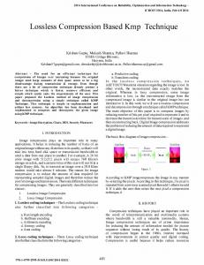
2.1. System Overview Figures 1 and 2 show block diagrams of the encoder and decoder, respectively. On the encoder side, audio samples are buffered and processed frame by frame. Each frame is divided into blocks of samples. Typically there is one block for each channel. Input data with out-of-range magnitude are normalized before further processed. Depending on the input file format, data is sent either directly into the lossless PCM coding module or floating point to PCM conversion module. After converting floating point data to PCM format, the generated PCM data and their corresponding floating point residue are compressed separately. Thus, for floating point sound file, its bitstream is a combination of compressed PCM data and floating point residue. Normalization info float A
Float2Int
Int2Float
float B
Float
Dynamic Range Control
Float or Interger?
Float Residue Condense Diff Data
Entropy Coding
Input sound file format info Bitstream Multiplexing
Integer Buffer Integer Residue
Predictor
Original
III - 1016
Estimate Coefficient Estimation + Quantization
Entropy Coding Code Indices
Quantized coefficients
Fig. 1. Encoder block diagram.
ICASSP 2004
➡
➡ In March 2003’s MPEG meeting, the lossless PCM coding module proposed by Technical University of Berlin [5] has been accepted as one of MPEG-4 lossless audio standard’s first reference models. Because of its excellent coding performance, it is adopted in our lossless PCM coding module in this work. The PCM coding module consists of three major building blocks, i.e. coefficient estimation and quantization, predictor, and entropy coding of integer residue. The basic version of the PCM encoder uses one sample block per channel in each frame. Optionally, each block can be subdivided into four shorter sub-blocks to adapt to transient segments of the audio signal. The encoder generates bitstream information allowing random access at intervals of several frames. Furthermore, joint stereo coding can be used to exploit dependencies between the two channels. For each channel, a prediction residual is calculated using linear prediction with adaptive coefficients and adaptive prediction order. The coefficients are quantized prior to filtering and transmitted as side information. The prediction residual is entropy coded using one of several differing Rice codes. The indices of the chosen codes have to be transmitted.
2.2. Bitstream Structure The general bitstream structure of a compressed file is shown in Figure 3. The bitstream consists of a header, compressed information of super-frames, any possible non-audio data, and a CRC checksum field. The header consists of the actual file header, followed by the header of the original sound file. Currently, the encoder only supports PCM wave files (*.wav) as input files, and the wave header is directly embedded in the data stream of the compressed file. Each super-frame is a random access unit. The field ”R” appears at the beginning of each random access unit (e.g. each M frames) and specifies the distance (in bytes) to the next random access unit. Any prediction related parameters need to be reset at the boundary of each random access unit. Remaining non-audio bytes of the wave file are embedded after the last audio frame. The CRC checksum is stored at the end of the compressed file. If non random access mode is selected by the users, the compressed data will be cascaded one frame after the other and put between the header and non audio data part. In addition, no ”R” field is necessary at the beginning of each frame data. Header
Superframe 1
File header
Wave header
Superframe 2
......
Superframe N
Non audio data
CRC
Normalization info
R Entropy Decoding
Float residue
Sound file format info Float or Integer?
Bitstream
Demultiplexing
Float
Frame 1
Frame 2
......
Frame M
Expanding Diff Data
Int2Float
Dynamic Range Control
Integer part
Reconstructed sound
Float residue part
H_f
Compressed floating-point residue data
Integer
Entropy Decoding
Integer Residue
Estimate Code indices
H_i
Prediction
Channel 1
H_i
Channel 2
or Quantized coefficients
H_i1
Fig. 2. Decoder block diagram.
Ch 1.1
Ch 2.1
H_i2
Prediction data
Ch 1.2
Ch 2.2
H_i3
Ch 1.3
Ch 2.3
H_i4
Ch 1.4
Ch 2.4
Compressed integer residue data
Fig. 3. Bitstream architecture. For floating-point input files, their samples need to be first truncated to integer. The floating-point residue data is generated byte-wisely by finding the difference between the original normalized floating-point samples A and the truncated integer samples in floating-point format B. In this way, any possible calculation error caused by simple floating-point domain subtraction can be avoided so that perfect reconstruction at the decoder side can always be guaranteed. After eliminating unnecessary bits, the floating-point residue data is then packed and entropy coded. A multiplexing unit finally combines all coded bits from the PCM encoder, floatingpoint residue encoder and other side information bits to form the compressed bitstream. The encoder also provides a CRC checksum, which is supplied mainly for the decoder to verify the decoded data. On the encoder side, the CRC can be used to ensure that the compressed file is losslessly decodable. The decoder is significantly less complex than the encoder. It first decompress the entropy coded integer residual and then using the predictor coefficients to calculates the lossless integer signal. If the original sound file is in floating-point format, the decoder also needs to decompress the floating-point residue and add them to the integer part. The normalization information is used at the end to restore audio data’s original dynamic range.
For PCM input files, each frame only contains an integer part. For floating-point input files, there is a floating-point residue part following the integer part. The integer part of each frame consists of one or four sample blocks for each channel, where each block has its own block header ”H”, carrying general information about the block (e.g. silence block, joint stereo difference block, etc.). The block itself typically contains the prediction data and the compressed integer residual values. The floating-point residue part contains a header and compressed floating-point residue data. The floating-point part header contains necessary information to decode the floating-point residue. The residue data is a compressed version of the exponent and mantissa difference of each sample. 2.3. Byte-wise Difference Instead of doing a floating-point subtraction, we generate the difference between the floating-point samples A and B byte-wisely so that perfect reconstruction can always be guaranteed. Figure 4 illustrates how the byte-wise difference is taken for one data sample. In our implementation, there is no need to record the difference of the sign bit because all sign bits are kept the same after format conversion. The exponent and mantissa differences, denoted
III - 1017
➡
➡ IEEE float A
1 s1
8
23
e1
f1 lsb msb
msb IEEE float B
lsb
1
8
23
s2
e2
f2 lsb msb
msb 8 D(e)=e1-e2
Diff=A-B
msb
• The number of non-zero bits in D(f ) can be calculated implicitly.
lsb 23 D(f)=f1-f2
lsb msb
lsb
Fig. 4. Byte-wise difference. by D(e) and D(f ), consist of 8 and 23 bits, respectively. They can be calculated either by bit-wise XOR or by a simple subtraction. Each sample’s difference data is stored in a 32-bit format, leaving one reserved bit for any possible need in the encoding process. 2.4. Format Conversion How the PCM and floating-point format conversion is handled has a great influence on the generation of floating-point residue data, which greatly affects the overall compression performance. s 16-bit PCM int M=(-1) x 7 s -15 IEEE float B=(-1) 2 x 7.0 s IEEE float A=(-1) 2-15x 7.xxx
Diff=A-B
D(e)=e1-e2=0
f2 7.0=(111.00...0) =2 2 x(1. 1100...0 ) 2 2 f2 2 7.xxx=(111.xx...x) =2 x(1. 11xx...x ) 2 2 2
Proposition If a sample in the intermediate PCM file has its magnitude greater than or equal to 2n−1 , but smaller than 2n (n > 0), then the highest n − 1 bits in D(f ) should always be zero. 2.5. Handling the Floating-point Residue
D(f)=f1-f2= 00 xx...x
n-1 n-1 n Generalization: if 2 < |M|