facilitate rapid functional recovery; (iii) need to ensure adequate levels of ...... their simplified PC-interfaces (USB-based vs. explicit data acquisition), making it.
A Low-Cost Framework for Individualized Interactive Telerehabilitation
by
Chetan Jadhav September 2004
A thesis submitted to the Faculty of the Graduate School of The State University of New York at Buffalo in partial fulfillment of requirements for the degree of
Master of Science
Department of Mechanical and Aerospace Engineering State University of New York at Buffalo Buffalo, New York 14260
This thesis is dedicated to my son, Sidh and wife, Bharati
ii
Abstract The goal of these research efforts is to develop architecture and algorithms for an inexpensive telerehabilitation framework that facilitates the individualized rehabilitation therapy of patients’ in their homes while being monitored periodically by a remotely located physiotherapist over the Internet. The intended audiences are patients with upperlimb (UL) dysfunction, secondary to a cardiovascular accident (stroke) or physical injury. The motivation for the creation and deployment of this framework comes from the congruence of several factors including: (i) increased occurrence of patients with such upper-limb dysfunction; (ii) need to establish a frequent motor-rehabilitation regimen to facilitate rapid functional recovery; (iii) need to ensure adequate levels of supervision for fastest recovery; and (iv) the need to overcome various logistics and cost constraints. The challenges include: (i) the significant variability of functional impairment within individual patients as well as the patient population (due to differences in demographics, age and recovery/degeneration); (ii) the specialty-labor-intensive nature of rehabilitation regimen; and (iii) critical need for objective (and preferably quantitative) measures-ofperformance with adequate specificity, sensitivity, accuracy and repeatability for analysis of patient performance overcoming the subjectivity/variability between therapists. In identifying and addressing the critical requirements for creation of such a framework, three broad research and development themes are examined in this thesis. These include: (a) Creation of a Sample Deployment Environment: A Networked Virtual Driving Environment example is used to identify various development/implementation issues, integrate various aspects within a common framework and serve as a convenient
iii
deployment method in the patient’s house; (b) Development of a virtual/computational biomechanical patient model: Quantitative computational models of the performance of the patient are obtained by automating the acquisition and processing of various quantitative sensor-based measurements. The focus in this thesis will be on developing a sound kinematic model, with close linkages to the underlying physiological model, and leveraging techniques of kinematic calibration in a biomechanical parameter identification context to estimate the kinematic parameters of patient's upper-limb skeletal system. Such a process not only enhances the quality of individualization possible but also can help effectively decouple the problem of diagnosis and prescription from aspects of the delivery; (c) Generation of algorithms for motion- and force-based active exercise assist: Successful performance of exercise involves control of motion and force interactions between the device and the patient while ensuring the stability of the overall interaction and most importantly patient safety. Methods from non-linear control theory, such as input-output and input-state linearization, are leveraged to create a general formulation for
computation
of
compensatory
motions
and
forces
in
creating
various
assistive/resistive exercises. Results from simulation studies and several case-studies are used to illustrate various aspects of these research issues.
iv
Acknowledgment I would like to thank my advisor, Dr. Venkat Krovi, for his mentoring, encouragement and assistance provided, not only during this thesis, but also during various phases of my academic endeavor at University at Buffalo (UB). I would also like to thank Dr. Bloebaum and Dr. Mayne, who deemed my work good enough to be on my thesis defense committee. Thanks to all the friends at UB for helping me on various occasions. Special thanks to CP, Rajan, Leng Feng, Pravin, Tao and SK for all the fun we had while researching in ARMLab. Finally, I express my sincere gratitude to family members; Aai, Babuji, Bharati, Sidh and Shamal. I have tested their patience by running way from my responsibilities for past two years. Continuous email interaction with my sister, Shamal, made me feel at home. Most of all I want to thank my wife, Bharati, for all her love and encouragement. I can understand all the trouble you have faced, for past two years, in my absence. This work is dedicated to you and our Sidh.
v
Table of Contents Abstract................................................................................................................iii Acknowledgment .................................................................................................. v List of Figures ................................................................................................... viii List of Tables ........................................................................................................ x
Chapter 1: Introduction................................................................................1 1.1 1.2 1.3 1.4
Motivation ................................................................................................. 1 Contemporary Telerehabilitation Practices............................................. 2 Proposed Telerehabilitation Framework ................................................. 3 Architecture of the Proposed Telerehabilitation Framework................. 4
1.4.1 1.4.2
1.5
Patient Interface......................................................................................... 5 Therapist Interface..................................................................................... 6
Proposed Research.................................................................................... 8
1.5.1 1.5.2 1.5.3
1.6
Creation of a Sample Deployment Environment ...................................... 9 Biomechanical Parameter Identification.................................................. 9 Exercise Assistance .................................................................................... 9
Organization of the Thesis ....................................................................... 9
Chapter 2: Background...............................................................................11 2.1 2.1.1 2.1.2 2.1.3 2.1.4
Motivation/Needs .................................................................................... 11
2.2
Need: Make it easily available to the patient (at home).......................... 11 Need: Individualization and Monitoring ................................................ 12 Need: Decision Support and Decision Deployment Tools...................... 12 Need: Computational Biomechanical Modeling .................................... 13
Underlying Themes in Research and Resulting Requirements ............ 14
2.2.1 2.2.2 2.2.3
Deployment in Non-Clinical Settings...................................................... 14 Individualization leveraging automation ................................................ 15 Parametric Framework for Modeling, Analysis and Deployment ......... 17
Chapter 3: Overall Telerehabilitation/Virtual Driving Environment Framework Implementation.......................................................................19 3.1 3.2 3.2.1 3.2.2
Other Computer-enhanced Rehabilitation Therapy Environments ..... 20 Hardware................................................................................................. 22
3.3
Force Feedback Wheel ............................................................................ 22 Rate Gyros ................................................................................................ 26
Software Implementation ....................................................................... 27
3.3.1 Interfaces to Force-Feedback Wheel ...................................................... 28 3.3.2 Post-processing of Acquired Data ........................................................... 29 3.3.3 Graphical User Interface (GUI) .............................................................. 30 3.3.4 3D Virtual Environment .......................................................................... 32 3.3.5 Network Socket Implementation between Patient and Therapist Interfaces.................................................................................................................. 35
Chapter 4: Biomechanical Identification ..................................................37 4.1 4.2
Parameter Estimation for Biomechanical Modeling ............................ 37 Upper Limb Kinematic Calibration........................................................ 40 vi
4.2.1 4.2.2
4.3
Calibration of Planar Four-Bar Mechanism.......................................... 42 Calibration of Spatial Four-Bar Mechanism ......................................... 45
4.3.1 4.3.2 4.3.3 4.3.4
Kinematic Calibration of Spatial Four-Bar Mechanism ...................... 53 Geometric Errors in between Two Frames ............................................. 54 Gross Geometric Error in the Completed Four-Bar Mechanism .......... 56 Linear Superposition ............................................................................... 57 A Least-Squares Algorithm for Kinematic Calibration.......................... 59
Chapter 5: Active Motion and Force Assist ..............................................62 5.1
Rehabilitation Exercise Regimen........................................................... 62
5.1.1 5.1.2 5.1.3
5.2 5.3
Classification Based on Use of Equipment............................................. 62 Classification Based on Nature of Assist ................................................ 65 Classification Based on Type of Manipulator Assist.............................. 66
5.3.1
Overview of Existing Manipulation Assist Methods/Approaches ........ 67 Implementation of Manipulation Assist ................................................ 69
5.4
A Simplified Example to Explore Motion and Force Assist .................. 71
5.4.1 5.4.2
Exercise Assistance................................................................................. 72 Input-Output Linearization for Motion Assistance ................................ 74 Input-Output Linearization for Force Assistance .................................. 80
Chapter 6: Disscusion/Future Work..........................................................83 6.1
Conclusion .............................................................................................. 83
6.1.1 6.1.2
Biomechanical Parameter Identification................................................ 83 Exercise Assistance .................................................................................. 84
6.2 Future Work............................................................................................ 84 References:......................................................................................................... 88
Appendix A: Appendix B: Appendix C: Appendix D: Appendix E:
DirectX Implementation..................................................94 Force Feedback Toolbox User's Manual .......................97 Car Dynamics Equations.............................................. 108 Socket Implementation ................................................. 111 Parameter Sweep Studies ............................................. 112
vii
List of Figures Figure 1-1: Telerehabilitation in the form of VDE .................................................. 4 Figure 1-2:(a) Patient Interface, (b) Virtual Environment and (c) Library of Exercises ........................................................................................................... 5 Figure 1-3: Network Communication between Patient & Therapist Interface ........ 7 Figure 1-4: Possible Analysis at Therapist Interface ............................................... 8 Figure 3-1: Telerehabilitation in the form of VDE ................................................ 19 Figure 3-2: Force Feedback Gaming Wheel [42]................................................... 23 Figure 3-3: Wheel calibration................................................................................. 24 Figure 3-4: Torque Calibration Results.................................................................. 25 Figure 3-5: MG100 Rate Sensors........................................................................... 26 Figure 3-6: Encoder reading before and after filtering........................................... 29 Figure 3-7: (a) Dial Implementation, (b) Virtual Spring-Damper ......................... 31 Figure 3-8: Virtual Driving Environment .............................................................. 33 Figure 3-9: Planar Model of Vehicle Dynamics .................................................... 34 Figure 3-10: Network Implementation (a) Using PyMat, (b) Using S-Function... 35 Figure 4-1: Human Upper-Limb Kinematic Model ............................................... 41 Figure 4-2: (a) Formation of a closed kinematic Loop in the transversal plane; and (b) parameters of the 4-bar mechanism........................................................... 42 Figure 4-3: Ratio of estimated link-lengths to true values with increasing measurement noise (a) 5%; (b) 10%; and (c) 25%. ........................................ 44 Figure 4-4: Simplified patient upper-limb and wheel model ................................. 46 Figure 4-5: Spatial four-bar mechanism with arbitrarily placed rate sensors ........ 47 Figure 4-6: Angular velocities (Twist) produced by rate-gyro in its inertial frame ......................................................................................................................... 48 Figure 4-7: Update of spatial four-bar w.r.t. its initial position ............................. 50 Figure 4-8: Two Link Calibration Example ........................................................... 61 Figure 5-1: Sample exercises as suggested by the National Stroke Association [1]: (a) To strengthen the muscles which straighten the elbow; and (b) To strengthen the shoulder muscles as well as those which straighten the elbow62 Figure 5-2: Model for human interaction with steering wheel............................... 72 Figure 5-3: Position Control Simulation ................................................................ 79 Figure 5-4: Output of Feedback Linearized Motion Controller ............................. 79 Figure 5-5: Results of Force Controller Implemented using Input Output Linearization ................................................................................................... 81 Figure 5-6: Variation in the Position of the System............................................... 82 Figure 6-1: Present Implementation ....................................................................... 85 Figure 6-2: Proposed Future Implementation ............................................................. 86 Fig. A-I: Toolbox Execution Structure................................................................... 94 Fig. A-II: mextd calss ............................................................................................. 96 Fig. C-I: Planar Model of Vehicle Dynamics....................................................... 108 viii
Fig. D-I: Network Implementation....................................................................... 111 Fig. E-I: Absolute tracking error vs. spring constant ........................................... 112 Fig. E-II: Absolute tracking error vs. damping constant...................................... 113 Fig. E-III: Absolute tracking error vs. damping constant .................................... 113 Fig. E-IV: Frequency tests (a) no force, (b) spring force, (c) damper force ........ 114
ix
List of Tables Table 3.1: MG 100 specification............................................................................ 27 Table 4.1: Percentage error in estimation of link parameters ................................ 44 Table 4.2: Calibration Parameters .......................................................................... 61 Table C.1: Vehicle Parameters ............................................................................. 110
x
Chapter 1: Introduction The overall goal of these research efforts is to develop the architecture and algorithms for an inexpensive telerehabilitation framework that extends the individualized interactive nature of traditional rehabilitation therapies to the patients’ homes. The intended audiences are the patients with upper-limb (UL) dysfunction, secondary to a cardiovascular accident (stroke) or physical injury. This framework is intended to facilitate the rehabilitation therapy of patients’ in their homes while being monitored periodically by a remotely located physiotherapist over the Internet, using a framework that leverages use of various commercial-off-the-shelf (COTS) equipment.
1.1 Motivation The motivation for the creation and deployment of this framework comes from the congruence of several factors. Stroke is considered the most common causative factor for the UL dysfunction in American adult population. It is estimated that in the United States alone, over 737,000 people experience new or recurrent stroke, each year, leading to motor disability and UL dysfunction. Direct cost, such as hospitals, physicians, and rehabilitation, add up to $17 billion. Indirect cost, such as lost productivity, totals $13 billion [1]. From 1979 to 2000, the number of Americans discharged from short-stay hospitals with stroke as the first listed diagnosis increased by 31.3 % [2]. Additionally, significant aspects of the patient’s activities of daily living tend to be severely disrupted due to such an UL disability, creating a significant reduction in overall quality of life. However, it is well established that a suitable motor-rehabilitation regimen can facilitate significant functional recovery so that the patient can become as
1
independent as possible [3]. Some of the requirements for a successful deployment of any rehabilitation regimen are as follows. •
First, there is considerable evidence that directly links functional recovery to the duration, frequency, regularity and intensity of the rehabilitation therapy [4, 5].
•
Second, the early and accurate diagnosis of the disease coupled with careful characterization of the level of functional impairment is important. Significant variation of functional impairment can be seen not only between different patients within the patient population (due to demographic or age-related differences), but also within the same patient over time due to recovery or degeneration [6-8].
•
Finally, by its very nature, most rehabilitation regimen (and especially newer techniques such as constraint-induced therapy), require ongoing attention and monitoring by a rehabilitation clinician and/or therapist. The outcome and duration of such therapy is dependent upon accumulated experience of the therapist.
Hence, the above requirements need to be taken into account in any proposed framework.
1.2 Contemporary Telerehabilitation Practices In recent years, leveraging the power of the Internet, real-time transmission of video has come to supplement audio and data transmission for telemedicine applications in general, and telerehabilitation in particular. Many research groups [9, 10] are evaluating the effectiveness of this technology for conducting assistive technology assessments
2
remotely. In a representative scenario, the clinic-based telerehabilitation expert observes patients at a remote site performing rehabilitation therapy tasks with the help of a professional or a family member. The real-time video component of video teleconferencing provides a visual and explicit exchange of information during this process with significant acceptance from both patient as well as therapists. However, multiple camera views may be necessary in this approach, for the therapist to recognize the patient's activity patterns, resulting in an expensive rehabilitation option because of the increasing infrastructure (cameras, network-bandwidth) requirements. While it alleviates the need for travel, by either patient or therapist, quantitative assessment of a patient’s performance is difficult with the video-conferencing infrastructure. Thus, such systems are unable to leverage the quantitative computational infrastructure to assist the diagnosis. Hence various research groups, interested in telemedicine applications, are considering augmenting video information with collected quantitative physiological information [11]. However, such approaches are being considered principally for the cardiac, respiratory and diabetes management, (and are not being explored in the telerehabilitation context considered in this thesis).
1.3 Proposed Telerehabilitation Framework This thesis seeks to address some of the challenges and issues that arise when low cost COTS therapy devices are coupled with rehabilitation therapy protocols opening up the possibility of widespread deployment as truly inexpensive home-based personalmovement trainers. Advances in miniaturization of processors, sensors and actuators has created a new
3
generation of smart embedded force-feedback products that can not only sense a person’s motions but also can apply forces during the performance of such motions. Numerous COTS force-feedback computer interface devices have been developed, primarily for gaming applications. However, they offer significant yet cost-effective functionality and performance. Such devices can serve as interfaces to stimulate the sense of touch and movement, as well as to create customizable patterns of active or passive motion and force assists to user motions. It is to explore such possibilities that a paradigm for remotely supervised telerehabilitation is being developed, in the form of a networked virtual driving environment (VDE) with force-feedback.
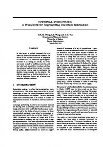
1.4 Architecture of the Proposed Telerehabilitation Framework
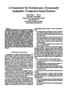
Figure 1-1: Telerehabilitation in the form of VDE The telerehabilitation framework under consideration, in the form of a VDE as shown in Figure 1-1, is being developed, to examine a network-based paradigm for assessment and rehabilitation of UL motor dysfunction while performing unilateral and bimanual 4
sensorimotor tasks. The overall framework consists of a Patient Interface (ultimately intended to be home-based) and a Therapist Interface (ultimately intended to be at a remote central hospital location) that are connected through the Internet. Each will be discussed in subsequent subsections. The emphasis is on the modularity and the bi-directional parametric coupling in all aspects of the development of this framework, which is intended
to
facilitate
“plug-n-play”
functionality
and
achieving
distributed
implementation, on different computational platforms located at different geographical locations. 1.4.1
Patient Interface
(a)
(b)
(c)
Figure 1-2:(a) Patient Interface, (b) Virtual Environment and (c) Library of Exercises The Patient Interface serves as both, the data-acquisition framework, as well as the exercise deployment framework. It consists of a virtual environment with which the patient can interact using a variety of COTS force-feedback kinesthetic interface devices. The focus is on selecting and validating the use of low-cost mass-produced devices and their simplified PC-interfaces (USB-based vs. explicit data acquisition), making it suitable for the Patient Interface. Other unobtrusively mounted sensors (such as MEMS rate Gyros mounted in a jacket) are also used to capture the users’ upper-limb motions. In 5
the longer term, it is proposed to include touch- and force-sensing film to monitor the hand contacts and inexpensive force torque sensors to measure the bilateral forces. As shown in Figure 1-2: (b), a variety of exercise scenarios, implemented in the form of driving activities within a virtual environment, forms the software component that is deployed on the patient’s home computer. At this stage, the overall framework is not significantly different from any of the commercially available networked interactive games. However, the addition of the parametric diagnostic and therapeutic modules sets the stage for creation of the individualized interactive therapeutic framework. As the patient interacts with the virtual environment, the diagnostic module captures the quantitative patient information (e.g. the pertinent motions and force histories) required for subsequent biomechanical identification process and for the development of performance measures (e.g. ranges of motion, measures of strength). A library of exercise routines created as specific parameterized driving scenarios (e.g. roads of increasing curvature, sharp turns as shown in Figure 1-2: (c) serves as templates to generate the desired exercise therapeutic regimen. The emphasis is on the parametric nature of the diagnosis and the subsequent therapy that form the cornerstone of these efforts. 1.4.2
Therapist Interface
A software package for human body simulation, JACK [12], is being used to develop the Therapist Interface. The digital human model, developed in JACK, will form the virtual prototype (“the avatar”) of the patient with which the therapist interacts within the Therapist Interface. The data collected at the Patient Interface, in the form of steering angle and gyro rates, is transmitted to the Therapist Interface over Internet. At the Therapist Interface, this data is used to update the arm pose of the digital model and the
6
position of the steering wheel. Figure 1-3 shows the conceptual network implementation.
Figure 1-3: Network Communication between Patient & Therapist Interface From the therapist’s point of view, this telerehabilitation system facilitates effective visualization and quantification of the patient’s motions and associated pathologies as the patient follows a prescribed exercise regimen. Digital human model consists of articulated rigid body models (69 scalable articulated parts, 138 degrees of freedom and 70 joints) that reflect the geometry and the kinematics of the patient [13]. Each such digital model will be customized to reflect the specific performance characteristics of each individual patient (ranges of motions and strength), as determined by biomechanical identification efforts (discussed later). The remotely collected data can be used to replay the patients driving (exercise) session on the digital human model and reviewed from various viewpoints. Furthermore, the interface can also provide the therapist with additional computed and postprocessed information (such as graphs of computed ranges of motion, comfort indices, etc., as shown in Figure 1-4) to aid the assessment process. The therapist can now appropriately modify the therapeutic regimen and download a new therapeutic regimen back to the patient’s machine. Accurate estimates of various patient kinematic parameters are required in order to customize the JACK model so that the exercise session recreated by the model resembles the actual patient performance. Furthermore, it is required to automate the process of link 7
length estimation to help reduce errors and increase the speed. The measured link lengths should be accurate enough to be used for further biomechanical analysis of patient's movements. The kinematic calibration techniques traditionally used in robotics will be adapted in this framework.
Figure 1-4: Possible Analysis at Therapist Interface
1.5 Proposed Research The overall framework, presented in the earlier section, has many areas that require careful attention in terms of research and development efforts. In this thesis, attention will be focused on three specific research and development issues described in following subsection.
8
1.5.1
Creation of a Sample Deployment Environment
This research aspect will help in identifying the issues with development, implementation and deployment of the overall framework. Additionally, it can help integrate many aspect of the framework in one common environment that will test the feasibility of the implementation of framework. 1.5.2
Biomechanical Parameter Identification
These research efforts are focused on identifying the kinematic parameters of UL. The techniques from robotics can be employed in identifying such parameters. Simulation studies of a simplified case and a more general case are investigated in this thesis. 1.5.3
Exercise Assistance
Various studies have shown that providing exercise assistance can aid functional recovery [14]. The research efforts in this part of thesis are focused on the investigation of use of nonlinear control method for providing exercise assistance. Simulation results of the developed controller will be discussed.
1.6 Organization of the Thesis In terms of general organization, the background literature for particular topic will be addressed in the corresponding chapters. This is intended to serve as an introduction to the corresponding topic and to motivate the subject matter immediately prior to presenting approach taken in the corresponding context. Chapter 2 motivates the need for telerehabilitation system by addressing merits and
9
shortcomings of contemporary rehabilitation practices. Functional requirements of the framework are identified and the fundamental research goals are evaluated in this chapter. Chapter 3 addresses the implementation of the framework in the form of Virtual Driving Environment as will serve to highlight the issues mentioned in Section 1.5.1. The hardware and software implementation and associated issues are discussed. Chapter 4 begins with the description of biomechanical parameters and motivates the need to identify such parameters in the context of individualization and performance evaluation. The later part of this chapter contains development of the kinematic parameter identification method, and simulation of it using planar and spatial four-bar mechanism. This serves to elaborate the issues discussed in Section 1.5.2. Chapter 5 expands the research and development issues that are identified in Section 1.5.3. Specifically, the use of method of nonlinear control theory to aid in the exercise performance will be explored here. Chapter 6 concludes the thesis with the list of contributions in this work and provides directions for the future work.
10
Chapter 2: Background The successful creation and deployment of the telerehabilitation framework, as envisaged in the previous chapter, raises a number of issues. This chapter first examines the motivations for creation and most critical needs of such a system, from among the many that exist. These identified needs will then serve to define both the broader underlying research themes as well as the specific sets of requirements desired by the overall framework with the goal of making such telerehabilitation approach, a viable alternative to traditional rehabilitation methods.
2.1 Motivation/Needs 2.1.1
Need: Make it easily available to the patient (at home)
As stated earlier, there is considerable evidence, which directly links functional recovery to the duration, frequency, regularity and intensity of the rehabilitation therapy [4, 5]. Many of these studies have confirmed that significant improvement is possible by following a dedicated therapeutic regimen (even several years after the initial incident). While the in-patient therapy remains the preferred means for stroke rehabilitation (in terms of recovery times), home-based rehabilitation programs have gained their importance and relevance. Such home-based programs afford considerable flexibility in tailoring the schedule, intensity and duration of the rehabilitation regimen while alleviating many of the economic issues related to the existing in-patient/out-patient rehabilitation facilities. Considerable literature has noted the benefits of home-based rehabilitation as a viable approach to provide treatment for stroke patients [15-17]. However, the logistics of such home-visits by the therapists/clinicians remains a 11
significant issue. 2.1.2
Need: Individualization and Monitoring
As mentioned earlier, significant variation of functional impairment can be seen not only between different patients in the patient population (due to demographic or agerelated differences), but also within the same patient over time due to recovery or degeneration [6-8]. Furthermore, newer techniques, such as constraint-induced therapy, have shown to bring about significant speedups in restoring the functional use [18-20] and to expand cortical representation of the exercised limb [21]. Evidence from studies on both acute and chronic stroke survivors has shown that the individualization in the form of “constraint-induced therapy” can improve movement ability with intensive and supervised training [18-22]. However, such a rehabilitation process tends to be labor-intensive, relying on diagnostic and therapeutic procedures that are administered by a qualified professional working with a single patient at a time. Therefore, by its very nature, any rehabilitation regimen needs to be individualized and requires the continued attention and monitoring from a rehabilitation clinician and/or therapist (relying on accumulated experience) for achieving the fastest recoveries. 2.1.3
Need: Decision Support and Decision Deployment Tools
Presently, therapists leverage their considerable experience and judgment while analyzing patient performance on an exercise regimen. However, by its very nature, such a subjective evaluation is prone to significant variability between therapists. There is a critical need for objective (and preferably quantitative) measures-of-performance with
12
adequate specificity, sensitivity, accuracy and repeatability for use in the analysis of patient performance. Such a quantitative framework, in conjunction with computerized analysis could also aid the creation of an automated decision-support system that can relieve the therapist from demanding task of such subjective evaluations. Similarly, there is a critical need for creation of a computerized and semi-autonomous framework for deployment of decisions without requiring direct therapist intervention at each step of the deployment. Thus, paralleling the developments in automation in several other fields, a computerbased sensor-enhanced analysis of patient performance coupled with a computerized semi-autonomous response deployment, with minimal therapist intervention, needs to be incorporated in the framework. 2.1.4
Need: Computational Biomechanical Modeling
Biomechanical modeling of the patient is a critical step for leveraging the computational capabilities of the overall system. Such a model can then serve as a surrogate affording the clinician/therapist the capability to interact and experiment in risky situations or in situations where the patient is not present. Such a model should therefore be created with adequate fidelity to reflect a patient's biomechanical characteristics and disease state and furthermore possess the capability to be updated in an ongoing manner to reflect changes. Developing accurate biomechanical model is an infinite dimensional problem due to complexity of physical systems and hence various approximations are used due to the finite computing power available. Thus, the framework should employ computationally efficient biomechanical model of a patient with adequate fidelity for automated analysis and decision-making.
13
2.2 Underlying Themes in Research and Resulting Requirements Many conflicting motivations and needs outlined in the previous section may be satisfied within the telerehabilitation framework as will be discussed in this section. In particular, wherever possible, the underlying theme will be expanded into sets of tangible requirements for deployment. 2.2.1
Deployment in Non-Clinical Settings The proposed telerehabilitation system is intended for individual use, with
minimal physical intervention from people other than patient. In particular, considerable emphasis is placed on the following aspects: •
The system leverages the use of COTS technologies to the largest extent possible. In doing so, the benefits of lowered costs and widest availability of various devices due to the mass-production are gained.
•
Emphasis is also placed on simplified computer-interfaces, for example, in terms of using the Universal Serial Bus (USB) is preferentially over dedicated dataacquisition (DAQ) cards. This is intended to leverage the ubiquitous home computer to which the additional hardware/software can be added even by untrained personal.
•
Finally, it is desired that, the overall system to be capable of being monitored over the Internet. The principal intent is to support the monitoring of patient exercise performance remotely as well as facilitating the remote updating of patient exercise regimen. At the same time, goal is to create a system that can operate with ubiquitously-available and non-dedicated devices, on limitedbandwidth variable-speed network environment that is characteristic of the 14
current day Internet, at low-cost. 2.2.2
Individualization leveraging automation
As noted earlier, motor-rehabilitation therapies tend to be labor-intensive, relying on diagnostic and therapeutic procedures that are administered by a qualified professional working with a single patient at a time. Such labor-intensive procedures are a primary application field for robotics and has resulted in development and deployment of robotassisted-therapy devices (“rehabilitators”) that physically-interact with patients in order to assist in movement therapy [23-26]. Such robotic devices now takes the role of a therapist in guiding the patient through the intensive and repetitive practice of functional movement, and several other studies have documented their successes [27-29]. In pursuing a similar approach within the proposed telerehabilitation framework, there are many levels, at which such individualization can be achieved and the focus is restricted to the following three aspects: •
At the very minimum, the computer-enhanced operation supports transparency of patient record-keeping, performance analysis and presentation of data to the therapist. For example, the system is intended to permit a quantitative and automated recording of patient performance (in raw form), which can be stored, retrieved, replayed and analyzed at subsequent times. Furthermore, such a system would simplify the monitoring of patient progress by permitting the analyst/therapist to retrieve and represent the patient data in a variety of forms. The digital revolution of the past several decades has promoted the trend towards
quantitative
monitoring
using
computerized
data
acquisition
technologies in general and the fields of rehabilitation and sports medicine are
15
no exception [30, 31]. •
At the next level, the computational framework is used to post-process and analyze the data. Such a post-processing serves to assist the data-reduction and elimination of spurious artifacts prior to transmission over a limited-bandwidth network. Additionally, the suitable development of measures-of-performance can leverage the available quantitative data to accurately assess the extent of the disease/therapy progress. Such an approach was adopted in the creation of various performance metrics for stroke patients performing bimanual manipulation tasks [32] and can be easily included within the proposed telerehabilitation framework.
•
However, the intent is to pursue the next level of individualization wherein the computerized measurements and computed metrics from the previous stages can be used to semi-autonomously modify the exercise regimen on COTS equipment. Such an effort requires increasing levels of automation, both in terms of execution of the assessment as well as in exercise delivery processes so that the exercise can be tailored depending upon a patient's disease state. The actual deployment of such a computer-controlled individualization operation can take two forms: (i) updated selection of a patient model or of the exercise parameters, typically from a parametric library, in response to measured performance with a previous selections in a lock-step iterative process; or (ii) online updating of parameters of the patient model or of the deployed exercise in response to measured performance during the performance of the exercise.
16
2.2.3
Parametric Framework for Modeling, Analysis and Deployment
The successful deployment of a “computerized measurement and therapy” system depends critically on the ability to acquire, manage and process information acquired from a patient and use this processed information to deploy the suitable therapeutic response. While automation is the key to managing this information flow, the intent here is to develop such automation within a parametric framework that is suitable for all stages of the information flow management. The complexity of biomechanical modeling has fostered the development of a number of approaches. For example, the simplest approach is to create lookup tables/phenomenological models that can serve as an approximation of exact biomechanical model. However, such lookup tables cannot adapt to the changing disease states of patient as they are based only on one observation of patient performance with out any theoretical basis. Furthermore, extensive preliminary examination will be required to make such lookup table for each patient. Alternately, the engineering community has used parametric models to serve as a finite basis and sought to approximate the infinite dimensional problem within such a basis. The coefficients now form the parameters describing the infinite dimensional problem in the region of interest. Similar approach can be employed in biomechanical modeling for the case in hand wherein the problem now reduces to parameter identification for which many sophisticated techniques, used by the System Identification community, are available. However, there are variety of bases that can be used – conventional polynomial, rational or alternately wavelet bases, to model multiple inputmultiple output interactions. Alternately, higher order models based on the kinematics
17
and dynamics of the underlying articulated structures could be leveraged to add more fidelity to the parametric identification problem – and it is this latter approach that will be adopt in this framework.
18
Chapter 3: Overall Telerehabilitation/Virtual Driving Environment Framework Implementation
Figure 3-1: Telerehabilitation in the form of VDE The telerehabilitation framework is developed in the form of a Virtual Driving Environment (VDE), shown in Figure 3-1. The intent is to examine such a network-based paradigm for assessment and rehabilitation of Upper Limb (UL) motor dysfunction while performing unilateral and bimanual sensorimotor tasks for the following reasons: •
First, it serves as an illustrative example to integrate the multiple facets of the research within a common overall framework for individualized telerehabilitation.
•
Second, it also allows identifying the issues with development, implementation and deployment of a flexible, reconfigurable, inexpensive, portable rehabilitation tool suitable for setup in patients’ home and outpatient clinics. 19
•
Finally, functional gains in driving activity are important for the disabled because it can extend their physical and social spheres of interaction and is vital for independent living. Hence, the development of such a rehabilitation tool, in the context of one of the higher activity of daily living (AsDL), can serve to enhance the motivation and compliance aspects of a therapeutic regimen.
However, this VDE is intended to serve as a network-based tool for assessment and rehabilitation of UL motor dysfunction and not necessarily as a “driving-simulator” for generic human-factor assessment or training [33]. In the following subsections, other similar computer-enhanced rehabilitation therapy environments are discussed prior to the detailed discussion of the hardware and software components of the infrastructure that combine to create the VDE.
3.1 Other Computer-enhanced Rehabilitation Therapy Environments The traditional goal for general computer enhanced rehabilitation environment has been immersivity, enhanced interactivity and transparency in data collection. Beginning in the late 1990’s, several researchers [14, 34-36] examined the application of robotic devices and automation technology to assist, enhance, quantify, and document neurorehabilitation. Hogan et al. [14] discussed the development and implementation of a robotic therapy device called the MIT MANUS, (a planar, two-revolute-joint robot) which assisted acute stroke patients in sliding their arms across a tabletop, and demonstrated the positive influence on the recovery process. Burdea and his co-workers examined many aspects surrounding the development, implementation and clinical testing of a home-based/PC-based orthopedic rehabilitation
20
system [37-39]. In [39], they introduce the use of the Rutgers Master II haptic device to serve as an instrumented interface to sample hand positions and provide suitable resistive forces. In [38], they enhance the system by including an alternative input device (cyber glove) and by setting up a set of immersive virtual environment based exercise protocols for hand movement studies. In [37], they extended the above therapeutic studies to detailed clinical trials with post-stroke patients in the chronic phase, as well as extending this concept for home-based ankle rehabilitation [40]. Reinkensmeyer et al. [25, 26] initially examined the development of a specialized robotic device, the ARM Guide. In addition to being a therapeutic tool, it also serves as a diagnostic tool, providing a basis for evaluation of several key motor impairments, including abnormal tone, incoordination, and weakness. As a therapeutic tool, the device provides a means to implement and evaluate active assist therapy for the arm. They also designed and tested a bimanual, lifting rehabilitator [41], acting on the presumption that specially designed rehabilitators automate some of the repetitive aspects of physical therapy and also improve them by responding more quickly and precisely than a human therapist and by quantitatively measuring a patient’s progress. Specifically, they built a device for assisting hemiplegic stroke patients in bimanual lifting as a part of developing a family of inexpensive machines, each designed to retrain coordination in a specific activity of daily living. However, the important contribution in the context of this thesis is in examining the use of a truly low cost, mass-produced COTS force-feedback devices (commonly used for gaming applications) for rehabilitation therapy applications. A modified COTS forcefeedback joystick (Microsoft Sidewinder) with an arm support was coupled to a target
21
tracking scenario to serve as an exercise protocol, implemented as a downloadable webbased, Java applet game [42]. While they examine the use of artificial assistive forces (generated via the force-feedback joystick) to favorably assist arm movements, they do not explicitly exploit the quantitative measurement capabilities of the low-cost setup to create a diagnostic tool. Apart from the case mentioned above [42], robotic therapy uses specialized devices, which are very expensive with limited ubiquitous access. Thus, it is in the final stages of bringing these advances over to the home-based rehabilitation arena that such approaches have faltered principally due to a combination of: (i) the lack of readily-available and affordable specialized equipment; and (ii) the lack of specialized/individualized therapies for each patient. The research efforts in developing this telerehabilitation framework focus on overcoming some of these limitations.
3.2 Hardware 3.2.1
Force Feedback Wheel
The Microsoft Sidewinder [43] force-feedback driving wheel (Figure 3-2), which is a very popular device used to give haptic feedback in computer games, is used as patient interface sensor as well as exercise delivery device. Force-feedback can add more realism to certain games by adding the sense of touch to the virtual world. Force-feedback wheels have most of the same components as ordinary gaming wheel, with a few important additions of an onboard 25 MHz microprocessor, an electrical motors and a gear train. The gear train transmits and amplifies the force from the motor to the steering shaft. Both an electrical signal from the onboard processor and the physical movement of the wheel
22
can rotate the motor axle. In this way, a user can still move the wheel even when the motor is moving it.
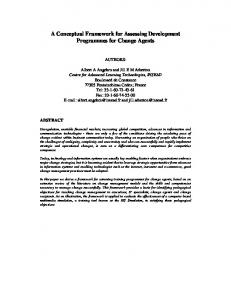
Figure 3-2: Force Feedback Gaming Wheel [42] On the opposite end of the motor, the axle is connected to the wheel's position sensors (a low-resolution optical sensor). Whenever the wheel moves, whether due to the motor or the player, the sensors detect its position. This wheel position is used to update the virtual environment as well as the force on the wheel. The wheel has a built-in ROM chip that stores various sequences of motor movement. For example, a damper effect which give resistance to patient's arm motions. The VDE requests a particular sequence, and the computer transmits the request to the wheel's onboard processor, which brings up the appropriate data from its own memory. This reduces the workload on the computer and allows faster reaction times. The wheel and the computer communicate using a simple USB interface, which makes it very easy to install on any computer with a USB port. The VDE controls the forces on the wheel using DirectX [44]. The device can exert a torque of ±1.87 N-m on the wheel axis with a range of motion of ±129o.
23
Impedance Calibration In order to maintain device independence, various inputs and outputs from DirectX are normalized. For example, the constant force effect applies torque ± 10000 units or steering angle is measured in ± 1000 units. The torque to be applied on steering axis is calculated using various Haptic Models as shown in Figure 3-7: b. Such a model requires angular velocities in rad/s and angular acceleration in rad/s2 of the steering axis. Further, output of such haptic model is the torque in N-m. Hence, it was essential to calibrate the steering wheel to convert DirectX units to physical units.
(a) Angle Calibration (b) Torque Calibration Figure 3-3: Wheel calibration Figure 3-3: (a) shows the angle calibration of the wheel. This is achieved by finding the steering range of motion. First, the diameter of the wheel is measured. The ends of the steering positions are marked on the periphery of the wheel and the distance between two marks is measured by placing a copper wire between the marks and measuring the length of the wire, which is 226 mm, as shown in Figure 3-3: (a). Using this arc length and the measured diameter the range axis rotation is calculated as:
24
226 × 2 2π − = 4.5078 rad 254.6
(3.1)
This range of motion corresponds to 2000 DirectX units. Hence, the angle calibration factor Ka is given by:
Ka =
4.5078 = 0.002253 rad DirectX Unit 2000
(3.2)
Torque Calibration 1.6
Torque N-m
1.4 1.2 1 0.8 0.6 0.4 0.2 0 0
2000
4000
6000
8000
10000
DirectX Units
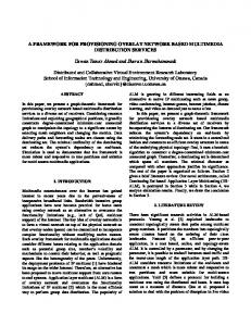
Figure 3-4: Torque Calibration Results For torque calibration factor, the experiment is set as shown in Figure 3-3: (b). A thin wire is wrapped around the periphery of the wheel. The wire is guided in to the slot on the periphery of steering wheel so that it is prevented from moving away from the periphery. One end of the wire is attached firmly to wheel and the other end is attached to weights. Experiment is started with a weight of 300 gm. The magnitude of constant torque effect in DirectX is gradually increased so that the torque applied by the device is balanced by the torque applied by weight. The experiment is conduced with increasing weights and the relationship between torque and DirectX units is found to be linear as 25
shown in Figure 3-4. The calibration factor Kt is found to be, K t = 1.873 × 10⁻⁴ N -m
3.2.2
DirectX Unit
(3.3)
Rate Gyros
Figure 3-5: MG100 Rate Sensors As human hand in conjunction with the driving wheel, forms a spatial four-bar mechanism with two degrees of freedom and details are given in Chapter 4 of this thesis. The wheel angular position is not sufficient to estimate the arm positions in space. Orientation of humerus and position and orientation of radius/ulna is essential to provide visual feedback, which is close to patient's arm movements, at therapist interface. This motivates to develop a sensor that can estimate the orientation of the arm. By considering the cost constraints of the framework, a low cost two d-o-f rate sensor MG100 by Gyration Inc. [45] is used in tandem as shown in Figure 3-5, to measure rotational velocities of body fixed reference frame. These sensors are commonly used in computer mice or remote controls and available with a considerably low cost. A unique electromagnetic transducer design and a single metal stamping utilize the Coriolis effect 26
to sense rotation. Analog voltages proportional to angular rates around the two sensed axes are provided relative to a voltage reference output. Its extremely low current consumption allows supplying power directly from PC eliminating the need for additional power source. Table 3.1 indicates some of the specification of the MG100 rategyro sensor. Parameter Sensitivity Supply Voltage Supply Current
Value 1.1 mV-s/deg 2.2-5.5 V 26-65 mA (peak) 5.4-10 mA (avrage)
Resolution
0.15 deg/s Table 3.1: MG 100 specification [45]
3.3 Software Implementation From the software perspective, the overall interactive environment is developed within a MATLAB/Simulink environment, leveraging various toolboxes, for example, GUIDE and VRML toolboxes can be easily leveraged to create immersive interfaces or various data analysis tools to perform analysis of data collected at patient interface. This greatly accelerates the initial implementation of the prototype framework. Additionally, MATLAB provides extensive functions to extend its capabilities in the form of Application Program Interface (API). The patient at patient interface is monitored using hardware described in section above. These devices are required to communicate with the graphical user interface (GUI), created in MATLAB/Simulink environment that provides visual feedback to the patient. In effect, the software interface at patient side is developed in two parts, hardware interface with the GUI and the GUI itself. Following subsection addresses these 27
software implementation aspects in details. 3.3.1
Interfaces to Force-Feedback Wheel
This interface is essentially required to access the force feedback device from MATLAB/Simulink environment. As the wheel has its own microprocessor and communicates with the PC using USB port, no additional data acquisition or motion control hardware is required to control the wheel. An application can access the wheel either by manufacturer supplied driver or through DirectX API [44] provided by Microsoft. This may not be a straightforward motion control, possible when explicit DAQ and motion control hardware is used, but offers incredible cost cutting when compared with the cost of DAQ hardware. MATLAB/Simulink provides a flexible extensible programming environment that enables to handle other non-traditional situations, where the existing capabilities of the MATLAB/Simulink can be extended. For example, MATLAB does not possess direct ability to control force feedback devices. However, it is possible to create an interface to access such a device leveraging the MATLAB external API. As mentioned earlier, one way of interfacing a force-feedback device with MATLAB is to call device driver functions in MATLAB API. Another option is to use DirectX in conjunction with MATLAB API. DirectX is a Microsoft Windows API that provides direct access to hardware, thereby helping mitigate time-delays inherent in a multitasking operating system. While it is developed with gaming applications in mind, it includes a library of force-feedback effect that is adapted in the framework. In particular, various effects can be composed together to create an entire library of assistive/resistive exercise regimen. Further details of this implementation are given in Appendix A:.
28
3.3.2
Post-processing of Acquired Data
Figure 3-6: Encoder reading before and after filtering The encoder mounted on the motor is of relatively low resolution and discretizes the wheel axis position in increments of 0.1 radians. It is important to obtain smooth estimate of the angular position, especially for subsequent estimation of velocities and acceleration by direct difference method. Since encoder signal does not contain random nose, a moving average filter was designed to smoothen the dicretization present in the acquired encoder signal as shown below: y[n] =
1 M
M −1
∑ x[n − k ]
(3.4)
k =0
where x is the raw encoder input to the filter, y is the filtered position estimate, M is the number of data pointes averaged in the filter, and n is the sample number. Figure 3-6 represents the encoder signal before and after filtering. In this case, the number of data points considered for moving average is 175 so that the filtered output is
29
smooth as well as not lagging. The filter is implemented using DSP blocks of Simulink. 3.3.3
Graphical User Interface (GUI)
The GUI reads quantitative patient information measured by hardware using the hardware interface described in the preceding section. These quantitative user-inputs are used to updates of the virtual environment according to an appropriate kinesthetic dynamic-interaction (haptic) model and to generate the motions and forces to be fed back to the user. A variable level-of-detail implementation is envisaged to facilitate mixing and matching the various levels of modeling and simulation fidelities – both for visualization (simple 2D GUI to detailed 3D environments) and haptic dynamic simulation (kinematic vs. dynamic vehicle models). Such an interactive environment can function in a standalone manner – in this form, it resembles any game that would be available on the market. Specifically, two implementations, with varying complexity of visual and haptic feedback to patient, are examined, including: •
A low complexity, rotary dial tracking experiment, essentially a 2D GUI as shown in Figure 3-7: (a).
•
A medium complexity 3D virtual driving environment as shown in Figure 3-8: (b).
The rotary dial tracking experiment is a single d-o-f rotational input motion tracking experiment. Dials and gauges from Simulink block library is used to implement this experiment as shown in Figure 3-7: (a). The desired orientation of the wheel is presented in the form of a light colored (red) needle and the current orientation of the wheel is indicated by the darker (black) needle. The desired orientation may now be made to
30
follow a variety of time-varying motions, which are tracked by the user. The squared norm of the angular difference between the desired and current orientation serves as a performance parameter.
(b)
(a)
Figure 3-7: (a) Dial Implementation, (b) Virtual Spring-Damper The haptic force-feedback to be provided to the patient is calculated using a single do-f torsional spring-mass-damper system as shown in Figure 3-7: (b). The governing equation can be written as: τ h = Iθ�� + Bθ� + Kθ
(3.5)
where, τ h is the torque applied by human, I is inertial of the wheel, K spring constant and B damping coefficient. I, K and B can have varying values and haptic model can have different characteristics. The basic requirement of such an impedance type haptic system is to read the current position from the steering wheel and apply measured torques on the wheel axis. The wheel is calibrated to acquire reading in radian and to apply torque in N-m as described
31
earlier. The various haptic system parameters such as K, B and I and motion parameters amplitude and frequency are also under control. A series of parameter sweep studies are performed with one human subject, wherein various values of the K, B, I are specified in the haptic model and the response is monitored as the human subject tracked a reference sinusoidal trajectory with varying frequencies. The goal is to determine the correlation between tracking error and parameters (K, B, I and frequency). It can be observed that there is no specific trend in tracking error for change in parameters K, B and I. Additionally, the average value of the tracking error (approximately 3 degrees) remains constant for all three experiments. These experiments indicate that the whole range of parameters is available for use in the exercises. From the frequency test, it can be concluded that frequency of the reference signal can affect the patient's tracking performance. To reduce this frequency effect, exercises can be created either with a constant frequency or with a very small frequency variation over stable range, which facilitates comparison of patient performance between different exercise sessions. The results are shown in Appendix E:. 3.3.4
3D Virtual Environment
This user interface is principally similar to dial experiment implemented in a form of vehicle driving task in virtual environment. The patient has to drive the vehicle near the center of the road. The deviation of the vehicle position from the center of the road serves as the performance parameter. In this case, road can have various shapes like sine or triangular wave. While driving on such curving roads, the patient get to exercises his arms and the amount of exercise can be controlled by changing road shape and force
32
feedback on the wheel.
Figure 3-8: Virtual Driving Environment The virtual environment is implemented using MATLAB Virtual Reality (VR) Toolbox. First, a static virtual environment is created using VRML as shown in Figure 3-8. This environment can be altered using VR Toolbox to produce animated visual feedback. Simulink reads the steering and pedal positions as inputs, which are used to solve car dynamics equations. Results of the solution are used to alter the virtual environment to provide visual feedback. The vehicle model, which also serves as haptic model for force-feedback, uses a simple yaw plane representation with three d-o-f [46] as shown in Figure 3-9 and the details are given in Appendix C:. The velocity and control vectors, in such a model, are defined respectively as: q� = U x U y uc = δ
Fxrf
Fxlf 33
r
T
Fxrr
(3.6) Fxlr
T
(3.7)
Figure 3-9: Planar Model of Vehicle Dynamics The driver input vector is given by:
ud = [δ
α
β]
T
(3.8)
where, δ is steering angle, α is throttle position and β is brake position. The corresponding acceleration and braking forces are assumed to be function of: Fad = f (α , q� )
(3.9)
Fbd = f ( β , q� )
(3.10)
For this thesis, a simple form is considered, where: Fad = K1α
(3.11)
Fbd = K 2 β
(3.12)
These driver inputs are mapped to control input by,
34
δ −F bd 4 −F bd uc = f ( ud ) = 4 Fad Fbd − 2 4 Fad Fbd 2 − 4
(3.13)
This haptic model can be considered as a block system, which takes input ud and produces the position, velocity and acceleration of the CG of vehicle and the force feedback that is proportional to the lateral yaw force on the front wheel. 3.3.5
Network Socket Implementation between Patient and Therapist Interfaces
(a)
(b)
Figure 3-10: Network Implementation (a) Using PyMat, (b) Using S-Function JACK has Python scripting interface through which a TCP/IP socket can be created for network communication. As mentioned earlier, MATLAB is used to create the Patient Interface. It is a scientific computing tool and does not contain any capability for network communication. Two approaches are tried to implement this network communication: (i) using PyMat Libraries as shown in Figure 3-10: (a); and (ii) Using MATLAB API as shown in Figure 3-10: (b). In first approach, the PyMat libraries are employed to create an interface between the MATLAB workspace and a Python application, which contains 35
a client socket. PyMat functions extract the data from the MATLAB workspace and the client socket, implemented in the same application where PyMat functions are used, sends that data to a server application scripted in JACK. The data received at the server is used to manipulate JACK model. Simulink has the C MEX S-Functions provision, as a part of MATLAB API, to use C code in the Simulink environment. Additional libraries can be included in S-Function and customized block can be created, to use with Simulink. Winsock2 libraries are used in C MEX S-Function to implement a client socket in second approach. As data is transmitted during every simulation cycle, this method was more robust and reliable since Simulink has total control over sending the data on network during every simulation cycle. The server socket is implemented in Python interface available with JACK similar to first approach. Details of implementation are given in Appendix D:.
36
Chapter 4: Biomechanical Identification
4.1 Parameter Estimation for Biomechanical Modeling Quantitative assessment and automation of monitoring holds considerable promise for not only enhancing the quality of individualization possible but also can help effectively decouple the problem of diagnosis and prescription from aspects of the delivery. In particular, three primary categories of motor patterns are used for assessing performance of movement tasks: •
Muscle activation or Electro Myographs (EMG) profiles provide insight into the coordination of muscle activation while performing a movement task;
•
Joint kinetics provide measures of the net causative demands placed on joint actuators (protagonist muscles) to perform a movement; and
•
Joint kinematics describes the necessary motion at the junction of inter-linking body segments required to accomplish a movement task.
The nuances of acquiring these three types of biomechanics measures in an accurate, valid and reliable way during human movement are well documented [47]. All three primary motor patterns used in biomechanics research are time-dependent and require some kind of frequency or time normalization procedures before averaging. For example, EMG signals from movement tasks are often converted to the frequency domain [48], time normalized and ensemble averaged [49], or subjected to statistical processing techniques [50] before they are compared to pathological movement patterns. Atypical motor patterns can then be identified by how much and when in the movement they differ from the normal patterns stored in databases. In some instances, a normal database might
37
not be required. When pathologies affect a single limb, the unaffected limb can be treated as normal for bilateral comparison between limb movement patterns.
This
method of within-subject comparison negates many of the confounding influences such as age, mass and height; however, time dependent signal normalizing techniques are still required. Bilateral comparisons are particularly powerful as an assessment tool and can often be reduced to a single measure such as the symmetry index [51]. In addition to direct measurements from the neurons, muscles, and limbs, considerable efforts in recent years have focused on developing computational models of the human neuro-musculoskeletal system. Developing such computational models is challenging because of the intrinsic complexity of modeling human motion generation, entailing the merger of cognitive, neural, skeletal and muscular subsystems, which must be represented accurately in order to provide insights into musculoskeletal performance. Efforts in recent years have led to the development of numerous parametric computational models ranging from artificial neural network-based models to relate upper limb movement to muscle EMG signals to full-fledged musculoskeletal modeling and analysis software such as SIMM [52] and Anybody [53]. However, generic models, developed using one of these software systems, need to be customized by adjusting its numerous parameters to match those of the specific individual – a process that can be tedious. However, given a model structure, considerable literature exists for parameter identification, especially in the context of online adaptive parameter estimation, which can be applied to good effect. In these efforts, focus is on adapting these techniques to aid the process of creation of customized models of the patients. The third category of motion patterns used for assessing movement task is kinematic
38
modeling. A suitable selection of both topology and various critical dimensions play a critical role in the creation and applicability of such kinematic model in biomechanical applications. First, such kinematic model forms a sound basis for many neuromuscular kinetic models because of their close linkages to the underlying physiology (articulated structure). Second, the selection of such topology (and thereby the nature of parametric model) can help minimize the number of parameters that may need to be determined. Finally, a sound kinematic model also forms a basis for graceful degradation of a kinetic model wherein the effects of actuators and masses are ignored. The focus in this thesis will be on developing such a sound kinematic model, with close linkages to the under lying physiological model. Developing an accurate patient's model is challenging because of the intrinsic complexity of biomechanical systems. For example, the forces produced by muscles depend on their activation, length, and velocity. Muscles transmit forces through tendons, which have nonlinear properties. Tendons connect to bones that have complex geometry and span joints that have complicated kinematics. Understanding how the nervous system coordinates movement is especially difficult because many muscles work together to produce movement, and any individual muscle can accelerate all of the joints of the body [54]. These complexities have important functional consequences and must be represented accurately if computational model has to provide insights into patient's performance. One approach in developing a patient's model is to customize the generic model (SIMM or Jack) with statistical averaged numerical values (e.g. skeletal measures) obtained from an anthropometric database [13]. However, the drawback of this approach
39
is that it is unable to capture the full extent of the variations between individuals. The alternate approach of non-invasive estimation using image-based measurements of skeletal parts from X-Ray, MRI or CT images has other drawbacks, including the need for multiple 3-D scans and extensive computations to determine kinematic quantities such as the center of rotation and the direction of its axis [55]. Hence, the proposed framework will use the ongoing and continuous streaming measurements to facilitate the automated and in-vivo estimation of various kinematic parameters of the upper-limb, building on the rich background of kinematic calibration in robotics [55, 56]. The accurate estimation of such parameters is especially important for the subsequent estimation of other quantities such as joint ranges of motion (and in the longer terms, the actuation forces at the joints). Such an accurate estimation is also important from the viewpoint of accurate visualization of patient's digital avatar. The end goal is a system that is capable of adaptively estimating these parameters based solely on the streaming measurements obtained with inexpensive COTS devices, without requiring expensive calibration tools.
4.2 Upper Limb Kinematic Calibration In this section, the use of techniques of kinematic calibration will be examined, specifically, to estimate the kinematic parameters of patient's upper-limb skeletal system. Approximating the patient's upper arm together with steering wheel a close-loop mechanism is formed. Modeling of the kinematics of the human arm offers considerable challenges since the considerable play in the mating joint surfaces combines with the surrounding tissue
40
deformation to result in complex motions. For example, the gleno-humeral joint (shoulder) acts like a cam and slides on the glenoid surface resulting in translation of the joint axis [57]. However, as an initial approximation, that is consistent with biomechanics literature, the human arm is modeled as an articulated kinematic linkage with 7 revolute joints as shown in Figure 4-1. A closed kinematic loop is formed when the patient then holds onto the driving wheel.
Figure 4-1: Human Upper-Limb Kinematic Model Two levels of approximations are considered to test kinematic calibration procedure: •
Simplified planar four-bar mechanism case; and
•
Spatial four-bar mechanism case.
Further details are discussed in the subsequent sections.
41
4.2.1
Calibration of Planar Four-Bar Mechanism
(a)
(b)
Figure 4-2: (a) Formation of a closed kinematic Loop in the transversal plane; and (b) parameters of the 4-bar mechanism For the purposes of initial kinematic calibration efforts, the motion of the arm is restricted to the transverse plane, parallel to the ground, passing through the shoulder as shown in Figure 4-2: (a). By assuming that that the torso of the patient is restrained by a seat-belt, the kinematics are reduce to that of a planar four bar mechanism, as shown in Figure 4-2: (b). A ground link, with unknown link-length l1 and unknown initial configuration Θ1 is assumed to stretch between the center of rotation of the wheel and the shoulder joint. The steering wheel forms the input-crank of known link-length l2 , the fore-arm is the coupler link of unknown length l3 and the upper-arm is the follower link of unknown length l4 . During the calibration process, it is assumed that the steering wheel encoder measures the relative joint rotations φ2 with respect to an (unknown) initial configuration Θ 2 . Similarly, the relative angular orientations, φ3 and φ4 with respect to (unknown) initial configurations, Θ3 and Θ 4 , are generated by resetting the
42
integration constant of the gyro-rate integration at the first calibration position. Thus the true joint angles may be written as θi = Θi + φi , ∀i = 2,3, 4 . Using the coordinates of the handgrip on the steering wheel as the point of interest, the difference between the measured and nominal approximated position may be written as: l cos θ 2 l1 cos θ1 − l3 cos θ 3 + l4 cos θ 4 ∆X = X measured − X nominal = 2 − l2 sin θ 2 l1 sin θ1 − l3 sin θ3 + l4 sin θ 4
(4.1)
In particular, θ 2 ,θ 3 ,θ 4 are considered to be the estimates solely due to the presence of the unknown initial configurations Θi , ∀i = 2,3, 4 . A Taylor series expansion of Eq. (4.1) in terms of variations of these unknown parameters can be written as Eq. (4.2), where Φ is calibration matrix and ∆ζ the vector of parameter variations.
cos θ3 ∆X = Φ∆ζ = sin θ3
− cos θ 4 − sin θ 4
−l2 sin θ 2 l2 cos θ 2
− l3 sin θ3 l3 cos θ 3
∆l3 ∆l 4 l4 sin θ 4 ∆Θ 2 − l4 cos θ 4 ∆Θ3 ∆Θ4
(4.2)
The calibration equations developed in Eq. (4.2) for a single position typically are undetermined. However, by making k such measurements for successive increments of φ2 , an overdetermined system of equations may be obtained as: ∆X 1 Φ 1 ∆ X = # = # ∆ζ = Φ∆ζ ∆X k Φ k
(4.3)
and a least-squares solution for the unknown parameter variations ( ∆ζ ) can be obtained by taking the pseudoinverse of this overdetermined system of equations.
(
T
∆ζ = Φ Φ
)
43
−1
T
Φ ∆X
(4.4)
2 L3 L4
1.5
Normalized Lengths
1 0.5 0 -0.5 -1 -1.5 -2
0
10
20
30
40
50
60
70
Iterations
(a)
2 L3 L4
Normalized Lengths
1.5 1 0.5 0 -0.5 -1 -1.5 -2
0
10
20
30
40
50
60
70
80
90
100
Iterations
(b)
2 L3 L4
Normalized Lengths
1.5 1 0.5 0 -0.5 -1 -1.5 -2
0
20
40
60
80
100
120
Iterations
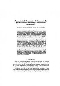
(c) Figure 4-3: Ratio of estimated link-lengths to true values with increasing measurement noise (a) 5%; (b) 10%; and (c) 25%. Lengths l3 l4 Iterations
% Length Error (5 % Noise) 4 0.3 43
% Length Error (10 % Noise) -2 -1 99
% Length Error (25 % Noise) 4 6 103
Table 4.1: Percentage error in estimation of link parameters 44
The estimated parameters l3 , l4 , Θ 2 , Θ3 , Θ 4 are updated using ∆ζ and the process is iterated for next set of k measurements until ∆X falls below a threshold ε . Results For the purposes of algorithm testing, a simulated 4-bar mechanism served as the source of measurements for φ2 , φ3 and φ4 . However, noting that the use of hobby electronic components in the final deployment is likely to give noisy measurements, the effect of the measurement noise is also investigated on online parameter estimation. Figure 4-3 depicts the results of the parameter estimation, while including the effects of addition of random measurement noise, ranging from 5% to 25% of the true value. Each subplot depicts the ratio of the estimated link-length to the true-value vs. the number of iterations. In general, the parameter estimation process converges rapidly for all cases but requires increasing number of iterations as the percentage of added noise increases. The results of these trials are also tabulated in Table 4.1. 4.2.2
Calibration of Spatial Four-Bar Mechanism
The preceding section has shown the special case of kinematic calibration with the assumption of the planar experimental setup and rate sensors that directly provide integrated angular measures. A more general case would be to model the patient's upperlimb and steering combination as a special spatial four-bar mechanism. Figure 4-4 represents a closed kinematic chain formed by patient arm and steering wheel. Only one arm is considered because of symmetry of the system. For simplicity, the shoulder joint is approximated as a spherical joint and the elbow and handgrip/wrist are approximated as a universal joint. Finally, the steering joint is treated as a revolute joint. Rate sensors are 45
attached at arbitrary locations on each moving link.
Figure 4-4: Simplified patient upper-limb and wheel model The degree of freedom of such a system can be calculated by: g
M = 6(n − g ) + ∑ f i
(4.5)
i =1
where M is the degree of freedom, n is number of moving links, g is number of joints and fi is the connectivity of joint i. The connectivity of spherical joint is three, that of the revolute joint is one and that of the universal joint is two. Therefore, connectivity of the arm-wheel chain is: 4
∑f i =1
i
= 1+ 2 + 2 + 3 = 8
(4.6)
As universal joint can be considered as two revolute joint connected by an intermediate link, number of moving link n is 5 and number of joints g is 6. Therefore, degrees-offreedom of the system is represented by eq.(4.5): g
M = 6(n − g ) + ∑ fi = 6 ( 5 − 6 ) + 8 = 2 i =1
46
(4.7)
This implies that two angle measures are adequate for complete pose determination of the arm-wheel chain. As rate sensors in the case in hand are arbitrarily placed on human arm, it cannot measure joint angle of human arm. Therefore, one three d-o-f rate sensor is used with each moving link of arm for determining orientation of the arm. Since, such a sensor is independent of joint configuration, the spatial four-bar mechanism can further be generalized as shown in Figure 4-5 with arbitrarily attached Gyros on each link.
Figure 4-5: Spatial four-bar mechanism with arbitrarily placed rate sensors Furthermore, Gyro output is angular velocities in its own moving frame the angular measures are obtained by integrating these velocities. Integrated results are dependent upon initial position of Gyro fixed frame and it is going to be different for every exercise session. Hence, it is required to calibrate the location of the sensor at the beginning of every exercise session. This calibration would require orientations of all the moving bodies. For kinematic calibration process, a forward kinematic equation of the
47
mechanism is required. Most of the forward kinematic representations require joint reading. As joint angles of human arm cannot be read by the rate sensors and its output is angular velocity vector in sensor fixed moving frame, a forward kinematic equation that can use such rate sensor readings is required. The following subsection elaborates the development of such a forward kinematic equation. Rate-Gyro reading conversion
Figure 4-6: Angular velocities (Twist) produced by rate-gyro in its inertial frame The matrices are denoted in square brackets and vectors are indicated by bold letter for the following development. The outputs of the Rate-Gyros are the angular velocity components of the twist vector, as expressed in the corresponding body-fixed moving frame. Output is the angular velocities, ω = ω x
ωy
T
ω z , in its inertial frame as
shown in Figure 4-6. Let R ( t ) ∈ SO ( 3) be the rotation matrix representing current orientation of gyro inertial frame w.r.t. initial orientation of that frame. Then the relationship between ω and R ( t ) is given by:
48
R� (t ) = [ R (t ) ][ Ω ]
(4.8)
where [ Ω ] is skew-symmetric representation of angular velocity vector ω and is given by: 0 [Ω] = ωz −ω y
−ω z 0 ωx
ωy −ω x 0
(4.9)
The solution of the differential equation is given by: Ωt R ( t ) = R ( 0 ) e[ ]
(4.10)
[R(0)] is identity matrix, because at t = 0, initial position of Gyro frame coincides with Gyro fixed moving frame. Hence, Eq. (4.10) becomes: Ωt R ( t ) = e[ ]
(4.11)
Eq. (4.11) can be solved using Rodrigues' Formula, which is: R ( t ) = e
= [I ]
[Ω]t
[ Ω] sin + Ω
( Ω t)
[ Ω] +
2
Ω
(1 − cos ( Ω t ) )
(4.12)
It is assumed that [ Ω ] is constant for each time step. The rotation matrix over a period of time T is given by:
[ R(T )] = [ R(t0 )][ R(t1 )]"[ R(tT )]
(4.13)
where [ R(t0 ) ] , [ R (t1 ) ] ," , [ R(tT ) ] are rotation matrices for corresponding time steps t1, t2,...tT. This rotation matrix captures the net orientation change due to the various angular rate motions w.r.t. the initial orientation of that frame. This net orientation change will be used together with the forward kinematics equation of the spatial four-bar mechanism in the subsequent kinematic calibration process.
49
Conversion of Absolute Orientation Changes to Relative Orientation Changes Consider the spatial four-bar in Figure 4-7 in two positions – an initial position and a position after time T. It is assumed the initial Gyros Frames {1}, {2} and {3} are coincident with joint centers at the initial position with their X-axis aligned along the length of the corresponding distal link at each joint. Frame {0} is the world coordinate frame. Frames {1'}, {2'} and {3'} are Gyro frames after a time interval tT. Gyro rates are integrated using Eq. (4.12) and Eq. (4.13) to give [R1], [R2] and [R3] ∈ SO(3), which represents rotation of current gyro frames {1'}, {2'} and {3'} w.r.t. its initial frames {1}, {2} and {3}, respectively.
Figure 4-7: Update of spatial four-bar w.r.t. its initial position The measured absolute orientation changes (as measured by Gyros) are required to 50
convert to appropriate orientation changes within the chain. Relative position of two frames can be described by: iTi +1 = iTi +1 [Qi +1 ]
(4.14)
where iTi +1 ∈ SE ( 3) refers to the initial position of Frame {i+1} as expressed in Frame {i}, and [Qi +1 ] ∈ SE ( 3) is the relative change from the initial position as expressed in Frame {i+1}. Furthermore, iTi +1 can be written as: i A iTi +1 = i +1 0
i
d i +1 1
(4.15)
where i Ai +1 ∈ SE ( 3) is the initial orientation of Frame i+1 w.r.t. Frame i and i d i+1 ∈ \ 3 is the translation from Frame {i} to Frame {i+1}. At this stage, the focus is solely on the orientation parts of these forward kinematic equations. Various integrated absolute orientation changes,
[ Ri ] ∀ i = 1, 2,3 ,
are all
expressed in inertial frames that happened to be installed at the initial position of the corresponding Gyro, as shown in Figure 4-7. A two-stage process is adopted to find the relative orientation changes of links within the chain based on these Gyro readings. Step I All these relative orientation changes are expressed in a common inertial frame, which is Frame {0}. Ri = 0 Ai [ Ri ] 0 Ai
−1
(4.16)
where, 0 Ai = 0 A1 1 A2 " i −1 Ai and k −1 Ak is the relative orientation of link k at
51
the initial position of the spatial four-bar. So by this token: R1 = 0 A1 [ R1 ] 0 A1
−1
R2 = 0 A2 [ R2 ] 0 A2 R3 = 0 A3 [ R3 ] 0 A3
−1
−1
(4.17) (4.18) (4.19)
Step II The complete forward pose kinematics equation for Frame {i+1} relative to Frame {0} can be written as: 0Ti +1 = 0T1 [Q1 ] 1T2 [Q2 ]" iTi +1 [Qi +1 ]
(4.20)
Note that at this stage this expression consist of 4 × 4 homogenous transformation matrices, where: i −1 A i −1T = i i 0
Rq1 0 di and [Q ]i = 1 1 0
i -1
(4.21)
Once again, considering only orientation:
0 Ri +1 = 0 A1 Rq1 1 A2 Rq 2 " i Ai +1 Rq ( i +1)
(4.22)
So for various links, the general orientation can be expressed as: 0 R1 = 0 A1 Rq1 0 R2 = 0 A1 Rq1 1 A2 Rq 2 0 R3 = 0 A1 Rq1 1 A2 Rq 2 2 A3 Rq 3 And various Rqi 's may be recursively solved as:
52
(4.23)
−1
Rq1 = 0 A1 0 R1
(4.24)
−1
Rq 2 = 0 A1 Rq1 1 A2 0 R2 −1
Rq 3 = 0 A1 Rq1 1 A2 Rq 2 2 A3 0 R3
4.3 Kinematic Calibration of Spatial Four-Bar Mechanism As noted earlier, the outputs of the Gyros are the angular velocity components of the twist vector, as expressed in the corresponding body-fixed moving frame. As such, the outcomes are independent of the actual sets of articulations within the underlying kinematic chain. The forward kinematic equation for the spatial four-bar now can be used to determine the pose of all members of the system. However, accurate estimation now depends both upon: (i) accurate estimation of initial pose of the system; and (ii) accurate updating of the relative change in pose based upon angular rate measures of the Gyro. Consider the calibration of serially connected four-bar mechanism as shown in Figure 4-7. Several aspects of the notation and formulation of [58] are adopted and extended the formulation to encompass the case of general rotation (and not simply rotations about a fixed axis). Let the base frame of the mechanism be zero. Then the forward kinematics of the four-bar is:
0T4 = 0T1 [Q1 ] 1T2 [Q2 ] 2T3 [Q3 ] 3T4
(4.25)
where 0T4 represents the position of the Frame {4} with respect to base frame. Kinematic calibration typically begins with a linearization of the forward kinematic equations. Let the nominal forward kinematics be
53
[T ] =
(
)
f T , [Q ] , where T
represent the initial positions and [Q ] is the relative change from the initial position. The linearized equation is of the form of: d [T ] =
∂f ∂f d T + d [Q ] ∂ [Q ] ∂ T
(4.26)
The differential, d [T ] , can be interpreted as the positioning error of the Frame {4} resulting from the kinematic errors that existed in T and [Q], so that it is equal to the difference between the theoretical position and the measured position of the Frame {4}. The kinematic calibration involves making several measurements of the error in the position of the Frame {4}, d[T], and determining the optimal d T , and d[Q] that minimize the error in the least-squares sense, e.g., minimizing: ∂f
∂f
∑ d [T ] − ∂ T d T − ∂ [Q ] d [Q ]
4.3.1
(4.27)
Geometric Errors in between Two Frames
Two assumptions are made in the development of calibration: 1. Small geometric errors exist in the initial position, T ; and 2. There are no measurement errors in the measurement of change in initial position, [Q]. Under these assumptions, all errors are lumped into errors in the initial position, T . Hence the term, ∂f
∂ [Q ]
d [Q ] , in Eq. (4.26) can be eliminated. Six geometric errors are
introduced into initial position, T . Since the parameters can fully describe the geometric errors, the calibration model is parametrically complete. The small error in the 54
initial position is defined to be d i −1Ti . This error can be realized by an infinitesimal translation
Trans ( dxi , dyi , dzi )
and
followed
by
an
infinitesimal
rotation,
Rot (δ xi , δ yi , δ zi ) , where dx, dy, and dz are infinitesimal displacements along x, y, and z-axis of Frame {i}, respectively, and δ xi , δ yi and δ zi are infinitesimal angles about x, y, and z-axis of Frame {i}, respectively. According to the definition of differential transformation: 1 0 Trans ( dxi , dyi , dzi ) = 0 0
Rot (δ xi
δ yi
1 δz δ zi ) = i −δ yi 0
0 1 0 0
0 dxi 0 dyi 1 dzi 0 1
−δ zi 1 δ xi 0
δ yi −δ xi 1 0
(4.28)
0 0 0 1
(4.29)
After adding the small error d i −1Ti , the corrected or measured position of Frame {i}, i −1Ti′ , relative to link Frame {i-1} becomes: i −1Ti′ = i −1Ti + d i −1Ti = i −1Ti ⋅ Trans ( dxi dyi
dzi ) ⋅ Rot (δ xi
δ yi
δ zi )
(4.30)
The differential transformation is expressed in Frame {i}. Hence, Eq. (4.30) follows the right multiplicative differential transformation of i −1Ti . Subtracting i −1Ti from both sides of the equation: d i −1Ti = i −1Ti ⋅ Trans ( dxi
dyi
= i −1Ti [ ∆i ] 55
dzi ) ⋅ Rot (δ xi
δ yi
δ zi ) − I 4×4
(4.31)
where: 0 δz [ ∆i ] = i −δ yi 0 4.3.2
−δ zi 0 δ xi 0
δ yi −δ xi 0 0
dxi dyi dzi 0
(4.32)
Gross Geometric Error in the Completed Four-Bar Mechanism
Now let us look at the gross geometric error between the actual position and the nominal position of the Frame {4}. For simplicity, it is assumed that the gross error can be realized by an infinitesimal rotation, Rot (δ x04 , δ y04 , δ z04 ) and followed by an infinitesimal translation, Trans ( dx04 , dy04 , dz04 ) , where δ x04 , δ y04 and δ z04 are the rotation angles about the axes of the base frame, and dx , dy , and dz are the displacements along the axes of base frame, respectively. It follows that 0T4′ = 0T4 + d 0T4 = Trans ( dx04
dy04
dz04 ) ⋅ Rot (δ x04 δ y04 δ z04 ) 0T4
(4.33)
The gross error, d 0T4 , is expressed in the base frame. Hence, Eq. (4.33) follows the left multiplicative differential transformation of 0T4 , and: d 0T4 = Trans ( dx04
dy04
dz04 ) ⋅ Rot (δ x04 δ y04 δ z04 ) − [ I ]4×4 0T4
= 0 ∆ 4 0T4
(4.34)
and 0 ∆ 4 = d 0T4 0T4 Similar to Eq. (4.32), 0 ∆ 4 is of the form:
56
−1
(4.35)
0 δz 0 ∆ 4 = 04 −δ y04 0 4.3.3
−δ z04 0 δ x04 0
δ y04 −δ x04 0 0
dx04 dy04 dz04 0
(4.36)
Linear Superposition
Based on the assumptions mentioned earlier, the errors in all the dyads contribute to the gross error of the position of the Frame {4}, d[0T4]. Thus, it can be written as a function of the errors of initial position of each link, d 0T4 . Since the geometric errors are all very small, the principle of linear superposition can be applied. It is assumed that the gross errors d[0T4] is the linear superposition of d i −1Ti . Let:
d 0T4 = d 0T4
(4.37)
where d 0T4 denote the differential errors of 0T4 due to the errors of initial positions. Then: 4
d 0T4 = ∑ 0Ti −1 i −1Ti′− i −1Ti iT4 i =1
4
= ∑ Ti −1 ⋅ d Ti T4 i −1
0
(4.38)
i
i =1
Eq. (4.38) sums up all the initial position errors of the dyads by first converting them into the base frame coordinates. Substituting Eq. (4.31) into Eq. (4.38), we get: 4
d 0T4 = ∑ 0Ti −1 i −1Ti [ ∆ i ] iT4 i =1
From Eq. (4.35):
57
(4.39)
−1
0 ∆ 4 = d 0T4 0T4 −1 4 = ∑ 0Ti −1 i −1Ti [ ∆ i ] iT4 0T4 i =1
(4.40)
Also, 0 ∆ 4 can be given by: −1
−1
−1
0 ∆ 4 = d 0T4 0T4 = 0T4′ − 0T4 0T4 = 0T4′ 0T4 − [ I ]
(4.41)
where 0T4′ is the actual or measured position of Frame {4} with respect to the base frame which is known and constant. If 0T4′ and 0T4 are sufficiently close, then 0T4′ 0T4
−1
is in the neighborhood of the identity matrix. Hence:
(
log 0T4′ 0T4
−1
) = ( T ′ T 0
−1
0
4
4
)
− [I ] −
(
−1
0T4′ 0T4 − [ I ]
)
2
2
+"
(4.42)
Using first order approximation:
(
0 ∆ 4 = log 0T4′ 0T4
−1
)
(4.43)
Because 0 ∆ 4 and [ ∆ i ] ∈ se(3) , they can also be represented as 6 ×1 vectors as follows: 0 ∆ 4 → 0 ∆ 4 = ( dx04
dy04
dz04 δ x04 δ y04 δ z04 )
[ ∆i ] → ∆i = ( dxi
dzi
δ xi
dyi
T
δ yi
δ zi )
T
(4.44)
Converting Eq. (4.40) into the adjoint representation: 0
4
∆ 4 = ∑ Ad 0T
i =1
(
Because log 0T4′ 0T4
−1
)
i −1
⋅ ∆i
(4.45)
is also an element of SE(3), it has a 6 × 1 vector
(
representation, denoted by log ∨ 0T4′ 0T4
−1
58
) . Combining Eq. (4.43) and Eq. (4.45) the
essential equation for calibration is obtained:
(
log ∨ 0T4′ 0T4
−1
)
4
= ∑ Ad 0T i =1
i −1
⋅ ∆i
(4.46)
Eq. (4.46) also can be expressed in the following form: y = [ A] x
(4.47)
where:
(
y = log ∨ 0T4′ 0T4
−1
)∈\
6×1
∆1 ∆ x = 2 ∈ \ 24×1 ∆3 ∆ 4 Ad 0T 1 Ad 1T 2 ∈ \ 6×24 A= Ad 2 T3 Ad 3 T4 The vector x contains the error parameters to be identified for the mechanism. The quantities in matrix [A] and 0T4
−1
are determined from the nominal model. 0T4′ can
be found from the actual measured data. 4.3.4
A Least-Squares Algorithm for Kinematic Calibration
To improve the accuracy of the actual model, the kinematic calibration procedure usually needs to measure the position of the end-effector in several different postures. In this case, because of close kinematic loop, position of end-effector frame is constant. For ith measurement, vector yi is obtained. The corresponding [Ai] can be determined from the nominal model. After several measurements, yi and [Ai] can be stacked to form the 59
following equation: Y� = A� x
(4.48)
where: T
y1 y � Y = 2 ∈ \ 6 m×1 # ym m = number of measurements x = error parameters in to be determined [ A1 ] [ A ] A� = 2 ∈ \ 6 m×24 # [ Am ] The least squares solution for x can be obtained by:
(
T x = A� A�
(
T where A� A�
)
−1
A�
T
)
−1
T A� Y�
(4.49)
is the pseudoinverse of A. The solution of Eq. (4.48) can be
further improved through iterative substitution. Let X denote the vector of the initial positions of the link attached frames and initialize X using the nominal model. Based on the measured data and Eq. (4.49), the error parameter vector, x can be obtained. The vector X is updated by substituting x into Eq. (4.30). The same procedure is repeated until the norm of the error vector, ||x||, approaches zero and the vector X converges to some stable values. Then X represents the final calibrated parameter vector.
60
Figure 4-8: Two Link Calibration Example A test example of this scenario was attempted considering the problem of kinematic calibration of a two-link planar RR manipulator as a trial case (Figure 4-8). The parameters of candidate mechanism used to generate the test data and parameters after calibration are listed in Table 4.2 Parameter
Initial
Calibrated
Actual
L1
1.2991
0.5942
0.6
L2
0.5
0.9972
1.0
Table 4.2: Calibration Parameters
61
Chapter 5: Active Motion and Force Assist In this chapter, some of the different ways in which manipulation resist/assist (both motion and force) may be provided in the context of rehabilitation are examined. Some of the current available classification methods for assistive and resistive exercises are surveyed. A general formulation of the problem is then presented and the issues pertaining to the computation of motions and forces required for the compensation in such system will be discussed. Furthermore, the specialization to an one-dimensional example of motion assist and torque assist in the driving scenario is investigated and the development of an exactly compensating control schemes for the motion- and force-assist scenario are discussed.
5.1 Rehabilitation Exercise Regimen 5.1.1
Classification Based on Use of Equipment
Unassisted Exercises
(a) (b) Figure 5-1: Sample exercises as suggested by the National Stroke Association [1]: (a) To strengthen the muscles which straighten the elbow; and (b) To strengthen the shoulder muscles as well as those which straighten the elbow Unassisted exercises have traditionally formed the mainstay of stroke rehabilitation therapies, especially in home-based settings. The National Stroke Association [1]
62
suggests some sample exercises for people who are (mildly) affected by stroke as shown in Figure 5-1. The disadvantages of this form of unassisted exercises are that not every patient is able to perform such exercises. Secondly, they might also not be motivated enough to carry out such “tasks”. Finally, the benefits from these exercises are minimal, as they do not appropriately stress the affected parts/muscle. Machine-Assisted Exercises The most effective rehabilitation regimen is to employ machine-assisted exercises to improve the functional capacity (and strength) of the affected skeletal muscles. Typically, such machines possess passive resistance/damping elements that act against the motion and forces created by the patient, thereby providing the exercise benefits. The kinematics of such machines can be customized/designed in order to realize a prescribed task space motion and forces. Such machine-assisted regimen can be used to realize a wide variety of exercise objectives including Isometric, Isotonic or Isokinetic [30, 31]. The digital revolution of the past several decades has been promoting the trend towards quantitative monitoring using computerized data acquisition technologies in general and the fields of rehabilitation and sports medicine are no exception [30, 31]. In recent times, several newer exercise machines known as Computerized Exercise Systems (CES) incorporate variability in the resistance or velocity of exercises, thereby making them adaptable to different users. Such CES tend to use computer control of passive resistive/damping elements to achieve their goals, which tends to limit the range of exercises possible. However, the principal benefits of such computerized data-acquisition systems stem from their ability to quantitatively, transparently and automatically monitor 63
(record/replay) various physical performance characteristics and perhaps most importantly to post-process (analyze/compare) the collected data. Robotic-Assisted Exercises Considerable attention in machine-assisted rehabilitation has focused on ConstraintInduced (CI) therapies. In Constraint-Induced therapy, the patient’s less impaired arm is restrained, and the patient intensively practices moving the more impaired arm, with feedback from the therapist [22]. Such a CI therapy approach has been shown to improve functional use [18-20] and expand cortical representation of the exercised limb. Evidence from studies on both acute and chronic stroke survivors have shown that the “constraintinduced therapy” can improve movement ability with intensive, supervised training [1826]. Several other studies have observed improvement in arm and hand movement ability after stroke with repetitive movement practice [28, 29, 59]. However, such therapies are also very labor-intensive, relying on diagnostic and therapeutic procedures that are administered by a clinician working with a single patient at a time. It must be noted that such labor-intensive procedures are a primary application field for robotics. Robot-assisted therapy refers to the use of robotic devices (“rehabilitators”) that physically-interact with patients in order to assist in movement therapy [23-26]. Similar results as that of constrained-induced therapy, are also seen in the robot-assisted therapy with additional benefits of improved quality, enhanced documentation and increased productivity [14, 24, 34, 35]. The robotic device now takes the role of a therapist in guiding the patient through the intensive, repetitive practice of functional movement. However, the significant costs and other logistics issues associated with using such devices make it possible to deploy these only in the hospital settings. 64
5.1.2
Classification Based on Nature of Assist
Passive Resist At the outset, note that the exercise equipment implementing principally resistive exercises using passive (or at the best semi-active) mechanical components such as dampers and spring have tended to predominate. Such an emphasis stems principally from the inherent stability of such passive system, which is important from the viewpoint of safety. Many of the computerized machine-assisted exercise systems tend to focus on computerized resistance adjustment. The principal drawback of such system is that they tend to be limited in terms of the range of motions and forces (as compared to those that would potentially be exerted by active equipment). Active Resist In recent years, several approaches have been considered for the use of actively controlled mechanical system for achieving suitable motion and force regulation. The creation of such system is of tremendous interest not only in the rehabilitation domain but also in wide variety of application such as haptic interactions with virtual environment and force-reflection in bilateral teleoperation applications. Active assist systems have significant limitations principally from the viewpoint of safety. All of the discussion to follow considers a robotic-assisted exercise wherein the patient interacts with the end-effector of a robot manipulator. While providing assist in the driving scenario, the steering wheel can be considered as a single link manipulator and a patient interacts with end-effector of such manipulator.
65
5.1.3
Classification Based on Type of Manipulator Assist
Motion Assistance The problem of providing motion assistance in a manipulation context can be treated as a conventional control problem of tracking a desired trajectory with the end-effector or regulating the end-effector of the manipulator to a desired set point. These trajectories/set points may be provided at the position, velocity or acceleration level. Traditionally, number of inputs must be at least equal the number of outputs in order for the problem to be nominally controllable. Force Assistance Alternately, instead of controlling the motion, as many force-related outputs as available inputs, can be targeted for control. At face value, while it may appear that simply one can replace motion control outputs with an equal number of force-control outputs. It is important to note that force control engenders certain innate challenges that are not typically encountered in motion control problem, as will be discussed later in this chapter. Combined Motion Force Assistance Multi-DOF articulated mechanical systems are excellent examples of multi-input multi-output systems where a mixture of motion and force objective needs to be met by the end-effector. Typically, such situation arises due to the addition of constraints to a multi-DOF multi-actuator system operating in free space. The goal is now one of controlling the motion in the space of feasible motions (which do not violate the
66
constraints) while simultaneously controlling the force interaction in the constrained directions. Principally such safety concerns arise due to the potential instabilities that are introduced due to the sampled data nature of control of the one or more actuators within such active system.
5.2 Overview of Existing Manipulation Assist Methods/Approaches Controllers designed for achieving a desired manipulation assist leverage several well-known approaches from robotics. For example, the motion assist can be formulated as a motion control problem for a robotics manipulator to find the set of joint torques which ensure that the end-effector can be either to follow a time-varying desired position and orientation, i.e. a tracking control problem, or to reach a constant desired position and orientation, i.e. a regulation problem. Similarly, a number of interaction-force control methods can be leveraged from robotics for this task. Such interaction-force control strategies can be broadly grouped in two categories: (i) performing indirect force control; and (ii) performing direct force control. The principal differentiating factor is that the former achieve force control via motion control without explicit closure of a force feedback loop. This category includes the compliance (or stiffness) control [60, 61], impedance control [62] among others. The direct force control methods afford the possibility of regulating the contact force to a desired value by means of closure of a force feedback loop. Traditionally, the inclusion of compliance between the robot and environment has played a significant role – such compliance may be introduced passively in the form of a suitable mechanical compliant device or actively by appropriate interaction control.
67
Compliance (or stiffness) control (or its dynamic equivalent impedance control) relate position error to the contact force through a mechanical stiffness or adjustable impedance parameters. Typical multi-DOF systems under impedance control are transformed into an equivalent mass-spring-damper system with the contact force as input. However, the resulting impedances, in the various task space directions, is typically nonlinear and coupled. If a force/torque sensor is available, then force measurements can be used in the control law to achieve linear and decoupled impedance. The selection of good impedance parameters that guarantee a satisfactory compliant behavior during the interaction may turn out to be inadequate to ensure accurate tracking of the desired position and orientation trajectory when the end effector moves in free space. Indirect force control schemes, such as compliance and impedance control are popular from the viewpoint that the force control problem reduces to the traditional motion regulation problem in the presence of environment interactions. Indirect control of the contact force, by suitably controlling the end-effector motion, ensures limited values of the contact force for a given rough estimate of the environment stiffness. Certain interaction tasks, however, do require the fulfillment of a precise value of the contact force. A radically different approach consists in designing a direct force control, which operates on a force error between the desired and the measured values. Direct force control on the other hand is more complex but can also be obtained by suitable modification of motion control schemes, i.e., by the closure of an outer force regulation feedback loop. Effective control often may require measurement of contact force. However, such a measurement process may be expensive both, in terms of sensor as well as additional computation.
68
However, decoupling necessitates the use of a force-torque sensor in the case of impedance control (even where force is not explicitly being controlled). Instead, the sets of measured contact forces may be put to better use to implement direct force control. A widely adopted strategy belonging to second category is the hybrid position/force control when a detailed model of the environment is available. This aims at controlling position along the unconstrained task directions and force along the constrained task directions. In most practical situations, a detailed model of the environment is not available. In such a case, an effective strategy still in the second category is the inner/outer motion/force control, where an outer force control loop is closed around the inner motion control loop, which is typically available in an industrial robot [63]. The problem of manipulation assist/control will be considered as the linear superposition of two sets of problems, a motion control problem and an interaction-force control problem. For tracking task, dynamic model-based state feedback compensation is required. For regulation of the end-effector to a constant desired and orientation, simpler control laws can be adopted, which do not require a full knowledge of the manipulator dynamic model, but just a static model-based compensation.
5.3 Implementation of Manipulation Assist Successful performance of exercise involves control of motion and force interactions between the device and the patient. Pure motion control often proves inadequate to control such interactions especially for performance of constrained exercises in the situations of incomplete modeling or in the presence of disturbances. One forthcoming advance in design of active exercise equipment is in enhanced integration of such active
69
interaction control capabilities. However there are many challenges to be overcome prior to adaptation of such active interaction control by the rehabilitation community. A few are discussed in the next few paragraphs. The dynamic model can be written in the Lagrangian form as: H ( q ) q�� + C ( q, q��) = τ − [ J ] h T
(5.1)
where q is ( n ×1) velocities of independent generalized coordinates used to describe the configuration of the overall system, [H] is ( n × n ) symmetric, positive definite inertia matrix, C ( q, q��) is the ( n ×1) vector of Coriolis and centrifugal torques, h = f T
µ T ,
where f denotes the ( 3 × 1) vector of external end-effector forces and µ is the ( 3 × 1) vector of external end-effector moments, and finally [J] is the
(6 × n)
end-effector
geometric Jacobian matrix, relating joint velocities to end-effector velocities. The dynamic model in the form of Eq. (5.1) is represented by a set of n second order coupled and nonlinear differential equations relating the joint positions, velocities and accelerations to the joint torques and the end-effector forces and moment. The actuator forces/inputs may be considered to be the sum of a motion assist component, τ m , and a force assist component, τ f , such that: H ( q ) q�� + C ( q, q��) = τ m and 0 = τ f − [ J ] h T
(5.2)
A position control scheme is implemented in the (constrained) motion space with τ m as the input and a force control scheme in the (constrained) force space with τ f as an input, resulting in the so called hybrid-control method. Notice, however such an orthogonal decomposition of motions and forces (and therefore development of controllers) is
70
relevant only in the joint-configuration space, which has the structure of a Riemannian manifold. 5.3.1
A Simplified Example to Explore Motion and Force Assist
Consider a simplified force control in one dimension M ( x ) �� x=u− f
(5.3)
The problem in Eq. (5.3) can be considered as a hybrid control problem as: M ( x ) �� x = um and f ( t ) = u f
(5.4)
However, this brings to light some of the fundamental problems with formulation and implementation of force control algorithms, i.e., when idealized actuator models are considered, the actuator inputs are related to the positions through a second order differential equation whereas these actuator inputs are related to output forces algebraically. This has some critical implications as follows: 1. There is a lack of causality between the inputs and outputs, which can create challenges in control; and 2. The actuators can at best statically compensate for the output forces (and never dynamically compensate for these force) due to the lack of dynamics in the actuator-input/output-force relationship. This aspect has been noted in the literature to limit applicability to quasi-static frameworks and hinders the implementation of full-fledged dynamic control. The solution has been to include some form of integral action for the reasons to be discussed below.
71
5.4 Exercise Assistance
Figure 5-2: Model for human interaction with steering wheel This subsection will address the modeling of the interaction of the human patient with the driving wheel and the virtual environment. Assume that the anticlockwise direction is the positive direction and consider the sets of parameters in the dynamics, as shown in Figure 5-2. The steering system is modeled as a second-order rotational spring-massdamper system, with an inertia J1 linear rotational damping constant B1, and a linear rotational spring parameter C1. With the assumption that this steering system is actuated by a torque τ act and is acted upon by an interaction force −τ int , the dynamics can be written down as: J1θ��1 + B1θ�1 + C1θ = τ act − τ in
(5.5)
Similarly, considering the human and other environment dynamics as forming a damped second-order system that can be written as: 72
J 2θ��2 + B2θ�2 + C2θ = τ h − τ in
(5.6)
Combining Eq. (5.5) and Eq. (5.6): + J 2 ) θ��1 + ( B1 + B2 ) θ�1 + ( C1 + C2 ) θ1 = τ act + τ h (�J�1 �
� � �
�� �
J
B
(5.7)
C
From Eq. (5.5): J1 τ act − Bθ�1 − Cθ1 − B1θ�1 − C1θ1 J J J J = 1 − 1 τ act + 1 B − B1 θ�1 + 1 C − C1 θ1 J J J
τ in = τ act −
(
)
(5.8)
The objective here is to propose a coordination framework that can be used to control the trajectory as well as interaction forces to the extent possible. The equations of motion are highly non-linear and coupled and the need to control the interaction forces further complicates matters. Note that only a formulation as a linear system is considered for convenience of explanation – the tools from nonlinear control, employed later in this section, can be applied with equal ease to the nonlinear problem as well. In the past, linearization about an operating point has been used to reduce the design of a controller to determining a linear state feedback – leading to unacceptable performance at points far away from the operating point. An alternative method is to employ nonlinear feedback linearization using differential geometric nonlinear feedback control methods. The states of the overall system can be written as: θ = θ 1 θ 2 θ 3 = θ1 θ�1 τ
(5.9)
Using the notation presented above the motion equations can be written in state-space form as:
73
θ2 θ�1 0 �2 C 1 B 2 θ 3 θ = − J θ − J θ + J + 0 u θ�3 1 0
(5.10)
= f (θ 1 , θ 2 , θ 3 ) + g (θ 1 , θ 2 , θ 3 ) u
5.4.1
Input-Output Linearization for Motion Assistance
In this first case, the output quantity to be controlled is considered the position of the system, hence the output equation may be written as: θ 1 y = [1 0 0] θ 2 θ 3
(5.11)
= h (θ 1 , θ 2 , θ 3 )
By writing the motion equations in the above form, an integrator in each input channel is introduced. This is to eliminate the direct input terms in the output equations. It is an affine system described by state Eq. (5.10) and the output Eq. (5.11). Nonlinear feedback linearization techniques may be applied to linearize the system if it is in fact known that the system is linearizable. There are several necessary and sufficient conditions regarding linearizability of affine nonlinear systems [64] that need to be checked for the present system. However, this process is very tedious – instead a nonlinear feedback can be derived. It can be verified that, this feedback does indeed linearize the system. The derivation of the nonlinear feedback requires the computation of the decoupling matrix, which can be performed as follows. Interested readers are referred to [64] for further details in the following process. Using the notation of differential geometry, the
74
Lie derivative of a function h(q) along a vector-field given by f(q) can be defined as: f1 ∂h ∂h ∂h L f (θ ) h = ⋅ f (θ ) = " # ∂θ ∂ θ ∂ θ n 1 f n
(5.12)
The second order Lie derivative of a function h(q) along a vector-field given by f(q) can be defined as: L2f = L f ( L f h ) =
∂ ( Lf h) ∂θ
⋅ f (θ )
(5.13)
Other higher order Lie derivatives may be defined similarly. The relative degree of the system may be defined as:
{
}
(5.14)
Lg ( LSf −1h1 ) Φ (θ ) = # S −1 Lg ( L f hk )
(5.15)
ρi = min s | Lg ( Lsf−1hi ) The decoupling matrix may then be defined as:
The current system under consideration has only one input, and hence only one output is considered at a time. The decoupling matrix may be computed by the method discussed above. Proceeding stage by stage, first calculating: 0 ∂h Lg h = g = [1 0 0] 0 = 0 ∂θ 1
(5.16)
Then calculating: Lf h =
∂h f ∂θ
75
(5.17)
θ2 C 1 B 2 θ3 = [1 0 0] − θ − θ + =θ2 J J J 0 0 Lg L f h = g = [ 0 1 0] 0 = 0 ∂θ 1
(5.18)
θ2 3 ∂L f h C 1 B 2 θ C 1 B 2 θ3 2 Lf h = f = [ 0 1 0] − θ − θ + =− θ − θ + J ∂θ J J J J J 0
(5.19)
∂L f h
∂L2f h
C Lg L h = g = − ∂θ J 2 f
B − J
0 1 1 0 = J J 1
(5.20)
Let:
[Φ ] = Lg L2f h det ([ Φ ]) =
1 ≠0 J
(5.21) (5.22)
The required nonlinear state feedback can be computed as noted below: u = α + βυ
[Φ ]α = − L3f h = −
C J
α=
−
B J
θ2 3 1 C 1 B 2 θ − θ − θ + J J J J 0
− BC 1 B B θ + C − θ 2 + θ 3 J J J
76
(5.23)
(5.24)
(5.25)
[Φ ] β = I
(5.26)
β=J
The relative degree of the system is three, which is also the dimension of the system. Thus, input-output linearization will also lead to input-state linearization. The states are transformed via a diffeomorphism which can be defined as: z = T (θ ) = h L f h L2f h z1 1 2 z = 0 z3 C − J
0 1 B − J
T
0 θ 1 0 θ 2 1 θ 3 J
(5.27)
(5.28)
z corresponds to the vector of new state variables in which the system is linear and the output is decoupled (but it also have a one-to-one correspondence with the original state variables, q ). The linearized system is described as: z�1 0 1 0 z1 0 2 2 z� = 0 0 1 z + 0 υ z� 3 0 0 0 z 3 1
(5.29)
The control system design in terms of this new linearized system can be easily done using pole-placement techniques as shown below: υ = z� 3d + K 2 ( z 3d − z 3 ) + K1 ( z 2 d − z 2 ) + K 0 ( z1d − z1 )
(5.30)
and the resulting control law in the original state-space domain can be calculated from this by stepping back through the diffeormorphism as: u = α + βυ (5.31) C B θ3 = Cθ 2 + B − θ 1 − θ 2 + + J z� 3d + K 2 ( z 3d − z 3 ) + K1 ( z 2 d − z 2 ) + K 0 ( z1d − z1 ) J J J
77
Note that the desired values in the linearized state (z) domain can be calculated based on the desired values of the original state variables using the diffeomorphism. z1d = θ 1d z 2d = θ 2d C 1d B 2 d θ 3d θ − θ + J J J � C B θ 3d = − θ�1d − θ� 2 d + J J J
(5.32)
z 3d = − z� 3d where,
θ 1d = Desired Position θ 2 d = Desired Velocity θ� 2 d = Desired Acceleration
(5.33)
θ 3d = Desired Force θ�3d = 0 Feedback Linearization
PID
J
C
B
K0
K1
K2
KP
KD
KI
10
15
25
6000
1100
60
2
0
0
Table 5.1: System Parameters Used in Simulation The performance of the system with and without manipulation assist controller are compared. For purposes of simulation, it is assumed that human motions results from action of any appropriate controller (PID, neural network, robust, MARC). In this thesis, it is assumed that this controller is of PID form. Table 5.1 gives the various parameters used for the feedback linearized system and the PID controller. Figure 5-3 demonstrated the results of simulation of position control of the steering system. Note that such a controller is unable to track the desired sinusoidal motions. In contrast, the feedback linearized motion controller is able to better track the desired reference.
78
Figure 5-3: Position Control Simulation However, the drawback of this approach is that the realization of the perfect tracking may require very high actuator forces as shown in Figure 5-4, which may not be realizable in all cases. Further analysis of the performance of this controller with the imposition of actuator limits is also possible but is one possible avenue for future work.
Figure 5-4: Output of Feedback Linearized Motion Controller
79
5.4.2
Input-Output Linearization for Force Assistance
In this second case, consider the controlled output quantities to be the interaction force exerted by the system. Hence, the output equation may be written as: θ 1 y = [ 0 0 1] θ 2 θ 3
(5.34)
= h (θ 1 , θ 2 , θ 3 )
Noting that the overall system may be written as: θ� = f (θ ) + g (θ ) u
(5.35)
θ2 0 C 1 B 2 θ3 where f = − θ − θ + and g = 0 . J J J 1 0 The appropriate Lie Derivatives can be computed as: 0 Lg h = [ 0 0 1] 0 = 1 1
(5.36)
The relative degree of system can now be computed to be 1. Note that when y=0, then q3 = 0, and the associated zero dynamics is: B C θ��1 = − θ�1 − θ 1 J J
(5.37)
which is asymptotically stable. Thus, the control law may be computed as: u=
1 − L f h − kh Lg h
80
(5.38)
θ2 C 1 B 2 θ3 where L f h = [ 0 0 1] − θ − θ + = 0 , and k is chosen such that the polynomial J J J 0 K ( s ) = s + k has all its roots in left half plane. If k = -1, then: 1 u = −0 − ( −1) θ 3 = θ 3 1
(5.39)
Hence, the control law can be written as:
u = θ�3d + K p (θ 3d − θ 3 )
(5.40)
Figure 5-5: Results of Force Controller Implemented using Input Output Linearization Figure 5-5 demonstrates the results of force controller simulation. The output of the force controller closely tracks the desired inputs. However, since the position is not directly controlled, it can change as shown in Figure 5-6, and may tend to drift.
81
As noted at the end of Section 5.3, the goal is to implement the overall manipulation assist as a combination of motion- and force-assist schemes discussed above. Efforts to this end are currently underway but are too preliminary to be reported in this thesis.
Figure 5-6: Variation in the Position of the System
82
Chapter 6: Disscusion/Future Work
6.1 Conclusion In this thesis, the various aspects of design development of a networked, low-cost home-based telerehabilitation system as an alternative to traditional rehabilitations methods are examined. Initially, the requirements and research issues associated with such a system were identified. Then, a scalable deployment framework for implementing such a system was proposed and demonstrated feasibility using a particular example of a Networked Virtual Driving Environment. This example not only helped to integrate various aspects of the research within a common framework, but can also serve as a convenient method for deployment in patients' houses without significant changes. Form technology point of view, several issues pertaining to integration of hardware and software were addressed in this thesis, which are discussed in chapter 3. From the research perspective, attention was focused on two major issues: biomechanical parameter identification and exercise assistance. 6.1.1
Biomechanical Parameter Identification
First, the planar case of four-bar mechanism was considered to show a simple example of identifying link lengths. The method was found to be robust for simulated sensor noise. Then, the arm pose determination using rate-gyros was investigated and developed a more general forward kinematic equation, for a spatial four-bar, which can use the rotation matrix measure produced by rate-gyro. Finally, a calibration algorithm for this spatial case was developed and tested with two-link mechanism. The algorithm was found to converge extremely quickly, often in less than three to five iterations. 83
6.1.2
Exercise Assistance
Various exercise methods and their classification according to various categories was discussed. Further, the assistive exercises were described and contrasted with resistive exercises. The methods from non-linear control were extended to develop exercise assistance for controlling both motion and force assistance scenarios. These controllers were tested and results are discussed in detail.
6.2 Future Work The implementation of the telerehabilitation framework offers many challenges of which this thesis addressed only a few. Some potential directions for future work are outlined below. •
The present calibration algorithm is solved using least square method. As the system requires estimating the parameters on an online basis, such a least square method may not provide real time performance. An estimation method based on recursive least square or Kalman Filter principle may work for ongoing estimation.
•
The design space of the calibration problem has many local minima and the solution obtained is nearer to the initial guess. In actual implementation, initial guess near to the actual parameters cannot be provided. Investigation in to a global method that can minimize from any arbitrary initial guess is required.
•
Present implementation of steering wheel involves real time computation architecture as shown in Figure 6-1. The major issue involved with such a system is the synchronization of sampling of steering wheel axis with solver running on
84
xPC system. Since host computer runs in Windows environment, variable sampling rate and TCP/IP connection between host and target computer, does not guarantee a real time data transfer. This does not guarantee accuracy of the results of numerical integration required in control algorithm implementation. Additionally, xPC needs a dedicated computer (in this case a PC/104 system) and the cost of such a system is prohibitive for home based installations.
Figure 6-1: Present Implementation This problem can potentially solved by implementing solver as a privileged or kernel mode application which uses the CPU time to solve the control algorithm. For example, Real-Time windows target kernel runs as a kernel-mode driver, intercepts timer interrupts from the PC clock, maintains clock signals for the Windows operating system, and ensures real-time execution of the real-time application. As a result, both the kernel and the real-time application run at CPU 85
ring zero. Though RT Windows Target can create a real time application in windows environment, there is no facility for communication between MATLAB running in non real time. Such a communication is essential to extract the output of the solver and use it in the main application. In future, an explicit kernel-mode driver that can communicate with the MATLAB application running in user mode (non real time) needs to be developed, as shown in Figure 6-2
Figure 6-2: Proposed Future Implementation •
In this thesis, the concentration was on kinematic parameter identification of upper limb. Several parameters are essential to define a biomechanical system completely. A thorough investigation in such parameters and sensor methods is required to implement the system as proposed in Chapter 1.
•
In the end, patient trials are required to test the effectiveness of the system.
86
Though the successful implementation of complete system may take considerable research efforts and time, it can be tested on a modular basis. For example, the assistive exercise part can be tested much before biomechanical identification part.
87
References: [1]
Anon. (2003). National Stroke Association. Available: http://www.stroke.org
[2]
Anon. (2003). Heart disease and stroke statistics 2003 update. American Heart Association. Available: http://www.americanheart.org
[3]
J. B. Reswick, "The moon over dubrovnik - a tale of worldwide impact on persons with disabilities," in Advances in external control of human extremities, 1990, pp. 4092.
[4]
G. Kwakkel, R. C. Wagenaar, T. W. Koelman, G. J. Lankhorst, and J. C. Koetsier, "Effects of intensity of rehabilitation after stroke. A research synthesis," Stroke, vol. 28, no. 8, pp. 1550-1556, 1997.
[5]
P. Langhorne, R. Wagenaar, and C. Partridge, "Physiotherapy after stroke: More is better?," Physiother Res Int, vol. 1, no. 2, pp. 75-88, 1996.
[6]
V. Krovi, "Design and virtual prototyping of user-customized assistive devices," Ph.D. Thesis, Department of Mechanical Engineering and Applied Mechanics, University of Pennsylvania, 1998
[7]
V. Krovi, V. Kumar, G. K. Ananthasuresh, and J.-M. Vezien, "Design and virtual prototyping of rehabilitation aids," Journal of Mechanical Design, Transactions of the ASME, vol. 121, no. 3, pp. 456-458, 1999.
[8]
V. Kumar, T. Rahman, and V. Krovi, "Customized assistive devices for people with motor disabilities," in Wiley encyclopaedia of electrical and electronics engineering, Ed. J. G. Webster, John Wiley & Sons, March 1999.
[9]
S. Dhurjaty, "Challenges of telerehabilitation in the home environment," presented at State of the Science Conference on Telerehabilitation, Washington DC, October 12-13, 2001.
[10]
J. Henderson, J. Lariviere, and K. Tran, "Optimizing assistive technology service delivery with video teleconferencing," presented at Technology and Persons with Disabilities, CSUN, 2000.
[11]
A. M. Cole and B. Q. Tran, "Home care technologies for an aging population," presented at State of the Science Conference on Telerehabilitation, Washington DC., October 12-13, 2001.
[12]
Anon. (2003). EDS Inc. Available: http://www.eds.com/products/plm/efactory/jack
[13]
N. I. Badler, C. B. Phillips, and B. L. Webber, Simulating humans: Oxford University Press, 1993.
88
[14]
M. L. Aisen, H. I. Krebs, N. Hogan, F. McDowell, and B. T. Volpe, "The effect of robot-assisted therapy and rehabilitative training on motor recovery following stroke," Arch Neurol, vol. 54, no. 4, pp. 443-6, 1997.
[15]
C. Anderson, S. Rubenach, C. N. Mhurchu, M. Clark, C. Spencer, and A. Winsor, "Home or hospital for stroke rehabilitation? Results of a randomized controlled trial : I: Health outcomes at 6 months," Stroke, vol. 31, no. 5, pp. 1024-31, 2000.
[16]
S. Byford, J. Geddes, and M. Bonsall, Stroke rehabilitation: A cost-effectiveness analysis of a placement scheme. York, UK: University of York, Centre of Health Economics, 1995.
[17]
J. B. Young and A. Forster, "The bradford community stroke trial: Results at six months," Bmj, vol. 304, no. 6834, pp. 1085-9, 1992.
[18]
S. L. Wolf, D. E. Lecraw, L. A. Barton, and B. B. Jann, "Forced use of hemiplegic upper extremities to reverse the effect of learned nonuse among chronic stroke and head-injured patients," Exp Neurol, vol. 104, no. 2, pp. 125-32, 1989.
[19]
E. Taub, N. E. Miller, T. A. Novack, E. W. Cook, 3rd, W. C. Fleming, C. S. Nepomuceno, J. S. Connell, and J. E. Crago, "Technique to improve chronic motor deficit after stroke," Arch Phys Med Rehabil, vol. 74, no. 4, pp. 347-54, 1993.
[20]
W. H. Miltner, H. Bauder, M. Sommer, C. Dettmers, and E. Taub, "Effects of constraint-induced movement therapy on patients with chronic motor deficits after stroke: A replication," Stroke, vol. 30, no. 3, pp. 586-92, 1999.
[21]
J. Liepert, H. Bauder, H. R. Wolfgang, W. H. Miltner, E. Taub, and C. Weiller, "Treatment-induced cortical reorganization after stroke in humans," Stroke, vol. 31, no. 6, pp. 1210-1216, 2000.
[22]
E. Taub, G. Uswatte, and R. Pidikiti, "Constraint-induced movement therapy: A new family of techniques with broad application to physical rehabilitation--a clinical review," J Rehabil Res Dev, vol. 36, no. 3, pp. 237-51, 1999.
[23]
D. Reinkensmeyer, N. Hogan, H. Krebs, S. Lehman, and P. Lum, "Rehabilitators, robots, and guides: New tools for neurological rehabilitation," in Biomechanics and neural control of posture and movement, Eds. J. M. Winters and P. E. Crago, Springer, New York, 2000, pp. 516-533.
[24]
D. J. Reinkensmeyer, L. E. Kahn, M. Averbuch, A. McKenna-Cole, B. D. Schmit, and W. Z. Rymer, "Understanding and treating arm movement impairment after chronic brain injury: Progress with the arm guide," J Rehabil Res Dev, vol. 37, no. 6, pp. 653-62, 2000.
89
[25]
D. J. Reinkensmeyer, B. D. Schmit, and W. Z. Rymer, "Assessment of active and passive restraint during guided reaching after chronic brain injury," Ann Biomed Eng, vol. 27, no. 6, pp. 805-14, 1999.
[26]
L. E. Kahn, M. L. Zygman, W. Z. Rymer, and D. J. Reinkensmeyer, "Effect of robot-assisted and unassisted exercise on functional reaching in chronic hemiparesis," in Proc. Engineering in Medicine and Biology Society, 2001. Proceedings of the 23rd Annual International Conference of the IEEE, vol. 2, pp. 1344-1347 vol.2, 2001.
[27]
C. Butefisch, H. Hummelsheim, P. Denzler, and K. H. Mauritz, "Repetitive training of isolated movements improves the outcome of motor rehabilitation of the centrally paretic hand," J Neurol Sci, vol. 130, no. 1, pp. 59-68, 1995.
[28]
H. M. Feys, W. J. De Weerdt, B. E. Selz, G. A. Cox Steck, R. Spichiger, L. E. Vereeck, K. D. Putman, and G. A. Van Hoydonck, "Effect of a therapeutic intervention for the hemiplegic upper limb in the acute phase after stroke: A single-blind, randomized, controlled multicenter trial," Stroke, vol. 29, no. 4, pp. 785-92, 1998.
[29]
R. Dickstein, Y. Heffes, Y. Laufer, N. Abulaffio, and E. L. Shabtai, "Repetitive practice of a single joint movement for enhancing elbow function in hemiparetic patients," Percept Mot Skills, vol. 85, no. 3 Pt 1, pp. 771-85, 1997.
[30]
Anon. (2003). Ariel Dynamics Inc. Available: http://www.sportscience.org
[31]
Anon. (2003). VERT Inc. Available: http://www.vertinc.com
[32]
P. Nair, C. Jadhav, and V. Krovi, "Development and testing of a low-cost diagnostic tool for upper limb dysfunction," in Proc. 2003 IEEE/RSJ International Conference on Intelligent Robots and Systems, Las Vegas, NV, United States, pp. 2600-2605 (IEEE cat n 03CH37453), 2003.
[33]
Anon. (2004). Systems Technology, Inc. Available: http://www.systemstech.com/stidrsm1.htm
[34]
H. I. Krebs, N. Hogan, M. L. Aisen, and B. T. Volpe, "Robot-aided neurorehabilitation," Rehabilitation Engineering, IEEE Transactions on [see also IEEE Trans. on Neural Systems and Rehabilitation], vol. 6, no. 1, pp. 75-87, 1998.
[35]
B. T. Volpe, H. I. Krebs, N. Hogan, L. Edelsteinn, C. M. Diels, and M. L. Aisen, "Robot training enhanced motor outcome in patients with stroke maintained over 3 years," Neurology, vol. 53, no. 8, pp. 1874-6, 1999.
[36]
B. T. Volpe, H. I. Krebs, and N. Hogan, "Is robot-aided sensorimotor training in stroke rehabilitation a realistic option?," Curr Opin Neurol, vol. 14, no. 6, pp. 745-52, 2001. 90
[37]
R. Boian, A. Sharma, C. Han, A. Merians, G. Burdea, S. Adamovich, M. Recce, M. Tremaine, and H. Poizner, "Virtual reality-based post stroke rehabilitation," in Proc. Proceedings of Medicine Meets Virtual Reality 2002, Newport Beach, CA, pp. 64 - 70, January 23-26, 2002.
[38]
D. Jack, R. Boian, A. S. Merians, M. Tremaine, G. C. Burdea, S. V. Adamovich, M. Recce, and H. Poizner, "Virtual reality-enhanced stroke rehabilitation," Neural Systems and Rehabilitation Engineering, IEEE Transactions on [see also IEEE Trans. on Rehabilitation Engineering], vol. 9, no. 3, pp. 308-318, 2001.
[39]
V. G. Popescu, G. C. Burdea, M. Bouzit, and V. R. Hentz, "A virtual-realitybased telerehabilitation system with force feedback," Information Technology in Biomedicine, IEEE Transactions on, vol. 4, no. 1, pp. 45-51, 2000.
[40]
M. Girone, G. Burdea, M. Bouzit, V. G. Popescu, and J. Deutsch, "Orthopedic rehabilitation using the `rutgers ankle' interface," in Proc. Proceedings of Virtual Reality Meets Medicine 2000, pp. 89 - 95, January 2000.
[41]
S. P. Lum, S. L. Lehman, and D. J. Reinkensmeyer, "The bimanual lifting rehabilitator: An adaptive machine for therapy of stroke patients," Rehabilitation Engineering, IEEE Transactions on [see also IEEE Trans. on Neural Systems and Rehabilitation], vol. 3, no. 2, pp. 166-174, 1995.
[42]
D. J. Reinkensmeyer, C. Painter, S. Yang, E. Abbey, and B. Kaino, "An internetbased, force-feedback rehabilitation system for arm movement after brain injury," in Proc. Proceedings of CSUN's 15th Annual International Conference: Technology and Persons with Disabilities, Los Angeles, CA, March 20-25, 2000.
[43]
Anon. (2004). Microsoft Corporation. Available: http://www.microsoft.com/hardware/sidewinder/Wheels.asp
[44]
Anon. (2004). Microsoft Corporation. Available: http://www.microsoft.com/windows/directx/default.aspx
[45]
Anon. (2004). Gyration Inc. Available: http://www.gyration.com/us/tech/technology.htm
[46]
J. C. Gerdes and E. J. Rossetter, "A unified approach to driver assistance systems based on artificial potential fields," Journal of Dynamic Systems, Measurement, and Control, vol. 123, no. 3, pp. 431-438, 2001.
[47]
D. Winter, Biomechanics and motor control of human movement, 2nd ed: John Wiley & Sons, Inc., 1990.
[48]
S. Karlsson, J. Yu, and M. Akay, "Time-frequency analysis of myoelectric signals during dynamic contractions: A comparative study," Biomedical Engineering, IEEE Transactions on, vol. 47, no. 2, pp. 228-238, 2000.
91
[49]
J. F. Yang and D. A. Winter, "Electromyographic amplitude normalization methods: Improving their sensitivity as diagnostic tools in gait analysis," Arch Phys Med Rehabil, vol. 65, no. 9, pp. 517-21, 1984.
[50]
M. P. Kadaba, H. K. Ramakrishnan, M. E. Wootten, J. Gainey, G. Gorton, and G. V. Cochran, "Repeatability of kinematic, kinetic, and electromyographic data in normal adult gait," J Orthop Res, vol. 7, no. 6, pp. 849-60, 1989.
[51]
S. C. White, L. A. Gilchrist, and B. E. Wilk, "Asymmetric limb loading with true or simulated leg-length differences," Clin Orthop, no. 421, pp. 287-92, 2004.
[52]
S. L. Delp and J. P. Loan, "A computational framework for simulating and analyzing human and animal movement," IEEE Computing in Science and Engineering, vol. 2, pp. 46-55, 2000.
[53]
J. Rasmussen, M. Damsgaard, E. Surma, S. T. Christensen, M. de Zee, and V. Vondrak, "Anybody - a software system for ergonomic optimization," in Proc. Fifth World Congress on Structural and Multidisciplinary Optimization, Lido di Jesolo - Venice, Italy, May 19-23, 2003.
[54]
F. E. Zajac, "Muscle coordination of movement: A perspective," J Biomech, vol. 26 Suppl 1, pp. 109-24, 1993.
[55]
R. N. Rohling and J. M. Hollerbach, "Modeling and parameter estimation of the human index finger," in Proc. IEEE International Conference on Robotics and Automation, vol. 1, pp. 223-230, 1994.
[56]
J. M. Hollerbach and C. W. Wampler, "The kinematic calibration index and taxonomy for robot kinematic calibration methods," International Journal of Robotics Research, vol. 14, pp. 573-591, 1996.
[57]
N. Palastanga, D. Field, and R. Soames, Anatomy and human movement: Structure and function. Oxford: Heinemann Medical Books, 1989.
[58]
I. M. Chen and G. Yang, "Kinematic calibration of modular reconfigurable robots using product-of-exponentials formula," Journal of Robotic Systems, vol. 14, no. 11, pp. 807-821, 1997.
[59]
C. Butefisch, H. Hummelsheim, P. Denzler, and K. H. Mauritz, "Repetitive training of isolated movements improves the outcome of motor rehabilitation of the centrally paretic hand," J Neurol Sci, vol. 130, no. 1, pp. 59-68, 1995.
[60]
R. Paul and B. Shimano, "Compliance and control," in Proc. 1976 Joint Automatic Control Conference, San Francisco, CA, pp. 694-699, 1976.
[61]
J. Salisbury, "Active stiffness control of a manipulator in cartesian coordinates," in Proc. 19th IEEE Confefence on Decision and Control, Albuquerque, NM, pp. 95-100, 1980. 92
[62]
N. Hogan, "Impedance control: An approach to manipulation: Parts i-iii," ASME Journal of Dynamic Systems, Measurement, and Control, vol. 107, pp. 1-24.
[63]
J. De Schutter and H. Van Brussel, "Compliant robot motion ii. A control approach based on external control loops," International Journal of Robotics Research, vol. 7, no. 4, pp. 18-33, 1988.
[64]
J. J. Slotine and W. Li, Applied nonlinear control, 1 ed: Prentice-Hall Inc., 1991.
93
Appendix A:
DirectX Implementation
As mentioned earlier that DirectX contains various types of effect types and effect modifiers. In the initial phases of development of telerehabilitation system, the use of these effects as assistive/resistive exercises is not known. Consequently, it was decided to implement the complete set of DirectX effect and it modifiers for MATLAB in the form of Force Feedback Toolbox, where a user can create and modify all the DirectX FFB effect from within MATLAB. With this toolbox, a user first creates a “force feedback effect” object in MATLAB. Parameters used to define such an objects in MATLAB are similar to those used to define DirectX FFB effect structure. Principally, Fig. A-I: Toolbox Execution Structure
a mirror-image of the DirectX FFB effect structure and associated methods was developed within the MATLAB
environment, which maintains these FFB objects in its workspace and also the corresponding DirectX FFB effect structure. A bidirectional update between the two is achieved using a DLL (a C++ mex-function). Thus all parameters of the DirectX FFB effect structure are accessible from and can be updated by simply updating the corresponding MATLAB object. This toolbox has a hierarchical execution structure as shown in Fig. A-I. MATLAB object oriented technique is employed to create effect objects in its workspace. At the 94
effect creation instance, methods of MATLAB effect object perform initial exception handling, creates a unique identifier (UID) for that effect and all the information including UID is sent to the DLL (directm.dll). Main role of this DLL is to resolve the command sent to it by MATLAB and call appropriate functions. The DLL receives all the input argument in the form of a pointer to a mxArray structure. When the DLL receives the command to create an effect, it calls the constructor of mextd class. This class receives the pointer to the mxArray structure, which the DLL has received as its input argument. MATLAB has provided extensive functions to extract the components of the received mxArray structure. In addition to that, utility functions that process the extracted mxArray data, so that it can be directly used to construct the DirectX effect structure are developed. Using MATLAB API functions and utility functions, mextd class creates DirectX effect structures. These structures remain as the part of the mextd class. When more than one effects are created, mextd class creates a linked list. Because of linked list data structure, there is no limit on the number of effects created. Correspondence between MATLAB effect object and mextd class, which contains all the effect information is established using the UID, generated in MATLAB effect constructor method. When application (Simulink model, MATLAB GUI or command form MATLAB command window) modifies the effect (start, stop, change effect parameters), corresponding MATLAB method does the initial error checking and passes the effect parameters to be changed and UID of the effect to be changed, to the DLL. The DLL polls through the linked list of the mextd class for the UID to find the desired effect to be modified and modifies that mextd class. When application terminates, the DLL frees the memory allocated to linked list and other DirectX structures.
95
Fig. A-II: mextd calss
96
Appendix B:
Force Feedback Toolbox User's Manual
97
Introduction This toolbox is intended to be used with force feedback (FFB) gaming devices. It can be used in MATLAB command window, MATLAB GUI or in Simulink as S-Function. A user can create a force feedback effect object in MATLAB workspace. Parameters used to define such objects are similar to those used in DirectX FFB effect structure. Matlab maintains these FFB objects in its workspace and also the corresponding DirectX FFB effect structure using a DLL (C++ mex-function). This DLL incorporates DirectX functions and creates a linked list of DirectX effect structures. The effect objects in MATLAB can be manipulated within MATLAB and the changes are reflected in the corresponding effect structure in DLL. Toolbox contains commands to start, stop, and modify an effect. Presently, this toolbox can create eleven types of DirectX force feedback effects with envelope structure. Additionally, the toolbox can read the X and Y angles of the device axis along with time stamp. Time information has adequate resolution to calculate time steps in microseconds. The time step can be used to estimate velocities and acceleration of the device axis. The toolbox has been successfully tested with Microsoft sidewinder force feedback devices. DirectX 9 is required for this toolbox.
98
Installation Unzip the downloaded file to some directory. Copy the DirectM folder from unzipped DirectM Toolbox folder to another directory, preferably the toolbox directory (matlabroot/toolbox/). Go to file menu in MATLAB window. Select Set Path submenu.
After selecting Set Path, Set Path window will open.
In Set Path window click on Add with Subfolder button. A browser 99
window will open.
In this window, select the directory where downloaded file is unzipped. Click OK. In Set Path Window, click Save and then Close button. After the installation procedure, toolbox command can be used in any working directory.
100
How to Use Irrespective of whether used in MATLAB or Simulink, the toolbox command should be called according to order given in the figure. Initialization
Effect Creation, Read
Effect Modification,
Termination When using in MATLAB command window, the order may not be followed and a user may experience unexpected errors. In such scenario use MATLAB command 'clear all' to terminate and initialize the toolbox again. While using with MATLAB GUI, the toolbox can be initialized in figure1_CreateFcn. Effects can be created or modified in various callback functions. Terminated the toolbox in figure1_DeleteFcn using clear all.
In
Simulink,
use
this
toolbox
in
M
S-Function.
Use
mdlInitializeSizes, mdlUpdate and mdlTerminate functions to maintain the toolbox execution order. mdlOutputs can be used
to read angles from the toolbox. Following commands can be used to control FFB devices in above mentioned order: Initialization Command: directm() Effect Creation: effect() Effect modification: start(), stop(), set() Read: directm() Termination: clear all (MATLAB command) Arguments to these commands are described in following section. 101
Command Reference directm Purpose
Start the DirectX and associate it with the application window
Syntax
directm('windowname') [x y t] = directm('read')
Argument
'windowname' is the name of the application window within
which toolbox is used. 'read' is used when axis position is required.
Description
DirectX requires a window handle to associate its effect structures. 'matlab' window name can be used for Simulink or MATLAB GUI applications. Passing 'read' argument to directm outputs the x and y axis positions in -1000 to 1000 range. t is the system time in seconds. Number of output arguments depends upon number of left side arguments to directm command while reading from the device.
Example
directm('matlab'); x = directm('read'); [x y] = directm('read'); [x y t] = directm('read');
102
effect Purpose
Create DirectX effects.
Syntax
effectobject = effect(duration,[envelope],'type', [type parameters], [axis direction]);
Argument
duration is the time for which the effect should run. It can be either 'inf' or time in microseconds. [envelope] is a 1 X 4 array describing the way effect should
start and end. The four parameters are: attacklevel Sets amplitude for the start of the envelope, relative to the baseline, in the range from 0 through 10,000. attacktime Time in microseconds to reach the sustain level fadelevel Amplitude for the end of the envelope, in the range from 0 through 10,000. fadetime Time in microseconds to reach the fade level The figure represents the enveloped applied to a sine effect.
An empty Passing [] empty array of envelope parameters sets NULL envelope. 'type' is the string describing effect type. effect can take
following effect types as an argument. These effect types are grouped as per DirectX convention. Condition effect type 'spring' 'damper' 'friction' 'inertia'
Periodic effect type 'square' 'sine'
103
'triangle' 'sawtoothup' 'sawtoothdown'
Constant force effect type 'constant'
Ramp force effect type 'ramp' parameters] are the corresponding parameters describing the 'type' mentioned above. These parameter are [type
different for different effect type. For condition effect type, [type parameters] are, offset Offset of the condition effect in the range from -10,000 to 10,000 positivecoef Coefficient constant on the positive side of the offset, in the range from -10,000 through 10,000 negativecoef Coefficient constant on the negative side of the offset, in the range from -10,000 through 10,000 positivesatu Maximum force output on the positive side of offset, in the range from 0 through 10,000 negativesatu Maximum force output on the negative side of the offset, in the range from 0 through 10,000 deadband Region around Offset in which the condition is not active, in the range from 0 through 10,000 For periodic effect type, [type parameters] are, magnitude Magnitude of effect in the range from 0 to 10,000 offset Offset of the effect in the range -10,000 to 10,000 phase Position in the cycle of the periodic effect at which playback begins, in the range from 0 to 35,999 period Period of the effect, in microseconds For constant force effect type, [type parameters] are, magnitude The magnitude of effect in range -10,000 to 10,000 For ramp force effect type, [type parameters] are, start Magnitude at the start of the effect, in the range from -10,000 through 10,000 end Magnitude at the end of the effect, in the range from -10,000 through 10,000 104
[axis] is a 1 X 2 array describing the direction in which effect is played on device. The two parameters are: xdir Describes the effect direction on x axis of the device. It can take values in the range -1 to 1. ydir Describes the effect direction on y axis of the device. It can take values in the range -1 to 1.
In case of steering wheel enter [1 0] so that the effect is applied on only one axis. In case of joystick apply effect on both the axis. For example, a axis parameter value [1 1] will play an effect in 45 degrees. Figure below gives an example of effect playback directions and corresponding axis values in case of Joystick.
[-1 1]
[1 1]
[-1 -1]
[1 -1]
Description
Many of the effect parameters can be changed using the set() command except the 'type' and [axis] parameters. Also once the envelope is set as NULL, it can not be changed. Please refer to DirectX documentation for further details about effect parameters.
Example
eff1
=
effect( duration, [attacklevel attacktime fadelevel fadetime], 'sine' , [magnitude offset phase period],[xdir ydir]);
eff2 = effect( 'inf',[],'constant', [10000], [1 1]); eff3 = effect( 'inf',[],'spring',[0 5000 5000 5000 5000 0],[1 0]); eff4 = effect( 'inf',[],'square', [10000 0 0 100000] ,[0 1]);
105
start Purpose
Start the effect
Syntax
start(effectobject)
Argument
effectobject is the effect created using effect command.
Description
After creating effect, it does not start by default. Use start command to playback the effect any time during modification phase. The effect object can be found in MATLAB workspace while using the toolbox in command window.
Example
start(eff2);
stop Purpose
Stop the effect
Syntax
stop(effectobject)
Argument
effectobject is the effect created using effect command.
Description
Use stop command to stop playing the effect any time during modification phase. The effect object can be found in MATLAB workspace while using the toolbox in command window.
Example
stop(eff2);
set Purpose
Modify the existing effect object parameters.
Syntax
effectobject = set(effectobject, 'parameter', newvalue)
Argument
effectobject is the effect created using effect command. 'parameter' is the parameter to be changed. newvalue is the value to be updated to 'parameter'.
Description
Following parameters can be changed. 106
'duration' 'attacklevel' 'attacktime' 'fadelevel' 'fadetime' 'offset' 'positivecoef' 'negativecoef' 'positivepatu' 'negativesatu' 'deadband' 'magnitude' 'offset' 'phase' 'period' 'magnitude' 'start' 'end'
Example
eff2 = set(eff2,'magnitude',5000); eff3 = set(eff3,'offset',8000);
107
Appendix C:
Car Dynamics Equations
The translational velocity Ux, Uy and angular velocity r of the car is given by: mU� x = Fxr + Fxf cos δ − Fyf sin δ + mrU y
(C.1)
mU� y = Fyr + Fxf sin δ + Fyf cos δ − mrU x
(C.2)
I z r� = aFxf sin δ + aFyf cos δ − bFyr + ∆Fxr
d d + ∆Fxf cos δ 2 2
(C.3)
Where Fxf = Fxrf + Fxlf
(C.4)
Fxr = Fxrr + Fxlr
(C.5)
∆Fxf = Fxrf − Fxlf
(C.6)
∆Fxr = Fxrr − Fxlr
(C.7)
Fig. C-I: Planar Model of Vehicle Dynamics
108
Assuming a virtual vehicle with throttle, brake and steer capabilities, the longitudinal forces and steer angle can be controlled so the equations of motion can be rewritten as, Dq�� = f (q� ) + g (q� , uc )
(C.8)
where the velocity and control vectors are defined as, q� = [U x U y uc = [δ
r ]T
Fxrf
Fxlf
Fxrr
ud = [δ
Fad
Fbd ]T
(C.9) Fxlr ]T
(C.10)
The driver input vector is givn by, (C.11)
where, δ is steering angle, Fad is throttle and Fbd is brake. These driver inputs are mapped to control input by, δ −F bd 4 −F bd uc = f (ud ) = 4 Fad Fbd − 4 2 Fad Fbd 2 − 4
(C.12)
Assuming equal slip angles on left and right tires, the longitudinal forces in the front and rear wheel is given by, U y + ra Fyf = −C f −δ Ux
(C.13)
U − rb Fyr = −Cr y Ux
(C.14)
where Cf and Cr are the front and rear cornering stiffnesses, respectively. All these
109
constants parameters assumed for the virtual vehicle is given by Table C.1. Parameter
Symbol
Value
Front cornering stiffness
Cyf
145,000 N/rad
Rear cornering stiffness
Cyr
145,000 N/rad
Front longitudinal stiffness
Cxf
300,000 N
Rear longitudinal stiffness
Cxr
300,000 N
Wheelbase
l
2.8 m
Distance from c.g. to front tire
a
1.37 m
Distance from c.g. to rear tire
b
1.43 m
Track width
d
1.5 m
Vehicle mass
m
1860 kg
Moment of inertia
Iz
3100 kg m2
Table C.1: Vehicle Parameters
In the Simulink implementation, the ud (3.8) is measured from the steering wheel and the throttle and brake pedals. From these inputs, uc (3.13) is calculated. The uc is used to solve the equations of motion (C.1), (C.2) and (C.3). The vehicle velocities [ q� ], obtained are in vehicle reference frame. These velocities are transformed to global coordinates using, X� cos (θ ) − sin (θ ) 0 U x � Y = sin (θ ) cos (θ ) 0 U y θ� 0 0 1 r
(C.15)
where X� , Y� and θ� are vehicle velocities in global coordinate system. After integrating these velocities during each simulation cycle, the VRML vehicle position is updated to provide the visual feedback to patient.
110
Appendix D:
Socket Implementation
Simulink has the C MEX S-Functions provision, as part of its API, to use C code in the Simulink environment. Winsock2 libraries in C MEX S-Function are used to implement a client socket. The server socket was implemented in Python. The user can enter server name or IP address, and the port number in the S-Function dialog box. This S-Function opens the socket to communicate to the given server and port number during the initialization of the Simulink model. Data is transmitted during every simulation cycle. The socket is closed during the termination of simulation.
(a) Server
(b) Client Fig. D-I: Network Implementation
111
Appendix E:
Parameter Sweep Studies
A series of parameter sweep studies were performed, wherein various values of K, B and I are specified in the haptic model and the response of the human subject tracking a reference sinusoidal trajectory with varying frequencies was monitored. The goal was to determine the correlation between tracking error and parameters (K, B, I and frequency). 10 9
Error (degree)
8 7 6 5 4 3 2 1 0 0
0.2
0.4
0.6
0.8
1
K (N/rad)
Fig. E-I: Absolute tracking error vs. spring constant The amplitude was fixed to be ± 1200, which is less than ± 1290, the range of motion of the steering wheel. Range of K, B and I constants of the DirectX effect is divided into five to six intervals. Experiment is conducted for each effect constant for 60 seconds. There was two-minute interval between experiments so that subject performance is not affected due to fatigue. Average error for each constant value is plotted against the corresponding value of effect constant. Fig. E-I, Fig. E-II, and Fig. E-III shows the absolute tracking error plotted against range of spring constant, damping constant and inertia respectively. It can be observed that there is no specific trend in tracking error for changing effects constants. Additionally, the average value of tracking error
112
(approximately 3 degrees) remains constant for all three experiments. 10
Error (degree)
8 6 4 2 0 0
0.1
0.2
0.3
0.4
B (N-s/rad)
Fig. E-II: Absolute tracking error vs. damping constant These experiments were conducted with a reference signal of 1 rads/sec frequency. Frequency tests were conduced to examine the effect of frequency on subject performance. In these experiments, frequency was increased form 0 to 2.5 rads/sec over a
Error (Degree)
period of 200 seconds.
10 9 8 7 6 5 4 3 2 1 0 0
5000
10000
15000
I (DirectX Units)
Fig. E-III: Absolute tracking error vs. damping constant Frequency tests were conducted with no force, spring force and damping force to examine the effect of force type as well. shows the results of these tests. It can be observed that irrespective of the force or force type the tracking error has significant influence of frequency of the reference signal. Error value increases moderately over 0 to 1 rads/sec frequency range. 113
(a)
(b)
(c) Fig. E-IV: Frequency tests (a) no force, (b) spring force, (c) damper force From the frequency test, it can be concluded that frequency of the reference signal can affect the patient's tracking performance. To reduce this frequency effect, exercises either with a constant frequency or with a very small frequency variation over stable
114
range can be created. This will facilitate us in comparing patient performance between different exercise sessions.
115