1
A machine learning approach to detect non-line-of-sight GNSS signals in Nav2Nav Monsak Socharoentum1*, Hassan A. Karimi2, and Yang Deng1
ITS- AP-SP0223 1National
Electronics and Computer Technology Center, THAILAND 2Geo-Informatics
Lab, university of Pittsburgh
[email protected]
Introduction - Non-Line of Sight Scenarios - Direct and reflected signals - Satellite group selections
2
Current solutions - Digital signal filtering techniques - Ge et al. (2000), Veitsel et al. (1998), Bétaille et al. (2003), Townsend and Fenton (2004), and Lee et al. (2004). - Hardware improvements - New antenna design Counselman, (1999); Boccia et al. (2004); Kamarudin et al. (2004); and Tatarnikov et al. (2005) - Laser scanner and inertial navigation system Soloviev and Graas (2008)
- 3D city model - Francois et al. (2011), Bourdeau et al. (2012), Groves et al. (2012), Obst et al. (2012a and 2012b), Wang et al. (2012), and Peyraud et al. (2013)
3
4
Proposed solution Pseudorange Correction Model and Algorithm
Open sky area
Station #2
Open sky area
Station #3
Station #1 Rover Urban canyon area
Station #n
Station and Rover receive same PRC from a satellite.
Station #4 Open sky area
Stations share PRC to Rover
Pseudorange Correction Model and Algorithm Phase 1
Phase 2
Phase 3
R1: Send request for help to all available Stations
S1: Calculate and map match its GPS position
R2: Average PRCs of each observable satellite
Rover
S2: Based on the map matched position, calculate PRC for each observable satellite S3: Send PRC to Rover
Station
R3: Calculate and map match Rover’s GPS position
R4: Based on the map matched position, calculate PRC for each observable satellite
R5: Classify satellite sets Rover
5
The experiment addresses two questions: • Is there a machine learning algorithm suitable for the problem? • Could the variables related to pseudorange measurement be used as predictors in the prediction model?
6
List of predictors for machine learning 1. Maxdiff:
the maximum of absolute PRC differences*;
2. Sumdiff:
the sum of all absolute PRC differences*;
3. SDdiff:
the standard deviation of absolute PRC differences*;
4. Maxtemp:
the maximum of all absolute PRC double differences**;
5. Sumtemp:
the sum of all absolute PRC double differences**;
6. PDOP:
the Position Dilution of Precision (the lower value indicates the higher probability to get better positional accuracy);
7. NSAT:
the number of visible satellites of each observation.
* PRC difference: Abs (PRCs of Rover - Average PRCs of Stations) ** PRC double difference: Abs (PRCs of Rover – 3* standard deviation of the PRCs of Stations)
7
Methodology and Simulation
8
• The learning phase: • Develop a prediction model
• The evaluation phase: • Examine the performance of the prediction model. 12.7 kilometers
4.8 kilometers Rover Station (learning phase) Station (evaluation phase)
Overall locations of Rover and Stations in the experiment
Methodology: learning and evaluation phases.
Simulation and Data Preparations
9
Table 1. Five scenarios in two phases. Scenarios
Numbers of stations
1 2 3 4 5
20 20 5, 15 5 5
Rover distance (kilometers) within cluster within cluster 10 4, 6, 8, 10 10
Magnitudes of signal delay (meters)
Time of observation
Phases
00:00; 2011-05-15 Learning Random Random 5, 20, 35, 50, 65, 80 13:00; 2014-02-16 Evaluation Random 5, 10, 15, 20, 25, 30, 35
Enumeration of data samples (notice that class 0 and 1 are imbalance) Data samples Phases Learning Evaluation
Class 0 (no multipath)
Class 1 (multipath exists)
Total
715
54,085
54,800
3,224
515,304
518,528
So, we apply cost-sensitive learning (CSL) technique (Witten et al., 2011)
10
Table 2. Performance of learning algorithms (for Learning phase). Learning Algorithms Methods no CSL Logistic Regression CSL* Support Vector no CSL Machine CSL* no CSL Naïve Bayes CSL* no CSL Decision Tree CSL*
0.999 0.938 1.000 0.934
0.061 0.967 0.000 0.981
0.976 0.975 0.500 0.957
Overall Accuracy 0.9875 0.9383 0.9875 0.9345
0.917 0.894 0.998 0.984
0.949 0.969 0.239 0.657
0.965 0.963 0.883 0.821
0.9173 0.8951 0.9883 0.9798
TP
Multipath exists
TN
No multipath
AUC
*use cost ratio FP:FN = 37:1
CSL does improve performance of True negative in three algorithms
Naïve Bayes performance for different rover distances TP
TN
11
Rover
Distance (kilometers)
AUC
Overall accuracy
A
4
0.965
0.976
0.989
0.9650
B
6
0.966
0.979
0.990
0.9659
C
8
0.946
0.980
0.984
0.9463
D
10
0.964
0.974
0.987
0.9643
The accuracies are all > 0.9, regardless of the distance
Naïve Bayes performance for different number of stations and magnitudes of signal delay Signal delay (meters)
5 20 35 50 65 80
Stations 5 15 5 15 5 15 5 15 5 15 5 15
TP 0.018 0.018 0.755 0.756 0.952 0.952 0.978 0.978 0.985 0.985 0.988 0.988
TN 0.974 0.973 0.974 0.973 0.974 0.973 0.974 0.973 0.974 0.973 0.974 0.973
AUC 0.695 0.703 0.944 0.944 0.983 0.982 0.990 0.990 0.992 0.992 0.993 0.993
Overall accuracy 0.241 0.244 0.7567 0.7573 0.9524 0.9523 0.9777 0.9778 0.9846 0.9846 0.9879 0.9879
The accuracies improve as the magnitude of signal delays increase
TP: Predict correctly that “multipath exists” TN: Predict correctly that “no multipath”
The performance drops quickly as the signal delay get close to the error of pseudorange measurement 7.8 meters at a 95% confidence (DOD, 2008).
Naïve Bayes performance against magnitudes of signal delay (5 stations; 10 kilometers Rover distance)
12
Conclusion • We present an alternative approach for identifying a satellite set containing a NLOS satellite in a cooperative vehicle environment. • Require PRC exchange between Stations (cars in open sky environments) and Rovers (cars in multipath prone environments) • The averaged prediction correctness rate are close to 90%. • Naïve Bayes algorithm has high TP and TN regardless of CSL (cost-sensitive learning). • Other algorithms (Logistic Regression, Support Vector Machine, and Decision Tree) perform poor prediction accuracy when CSL is not applied • The experiments show that a prediction model can be developed based on data from one location and time and used for a different location and time. • Station’s observations can be reused multiple times by multiple Rovers across a connected vehicle network.
13
14
Thank you
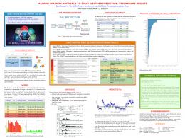
CSL needs weight ratio to resolve the imbalance class TP, TN, and AUC behaviors.
Using Logistic Regression
TP: Correctly predict “multipath exists” TN: Correctly predict “no multipath”
15