RankFrag: A Machine Learning-Based Technique for Finding Corners in Hand-Drawn Digital Curves Gennaro Costagliola*, Mattia De Rosa*, Vittorio Fortino†, Vittorio Fuccella* *Dipartimento di Informatica, University of Salerno, Via Giovanni Paolo II, 84084 Fisciano (SA), Italy †Unit of Systems Toxicology, Finnish Institute of Occupational Health (FIOH), Helsinki, Finland {gencos, matderosa, vfuccella}@unisa.it,
[email protected]
Abstract
in real time are crucial features for segmentation techniques. Tumen and Sezgin [26] also emphasize the importance of the adaptation to user preferences and drawing style and to the particular domain of application. Adaptation can be achieved by using machine learning-based techniques. Machine learning has also proven to improve accuracy. In fact, almost all of the most recent segmentation methods use some machine learning-based technique. The technique presented here, which we call RankFrag, uses machine learning to decide if a candidate point is a corner. Our technique is inspired by previous work. In particular, the work that mostly influenced our research is that of Ouyang and Davis [20], which introduced a cost function expressing the likelihood that a candidate point is a corner. We adopt their cost function, but our corner finding procedure is different. The technique works by iteratively removing points from a list of candidate corners. At each iteration, the point minimizing the cost function is classified and, in the case it is not a corner, it is removed. As a point is removed from the list, it is assigned a rank, which is a progressively decreased integer value. Points with a higher rank (a lower integer value) are more likely to be corners. Another important characteristic of RankFrag is the use of a variable “region of support” for the calculation of some local features, which is the neighborhood of the point on which the features are calculated. Most of the features used for classification are taken from several previous works in the literature [23, 15, 27, 21, 20]. Four novel features are introduced. We tested our technique on three different datasets previously introduced and already used in the literature to evaluate existing techniques. We compared the performance of RankFrag to other state-of-art techniques [28, 26]. Summarizing, this paper introduces and evaluates:
We describe RankFrag: a technique which uses machine learning to detect corner points in hand-drawn digital curves. RankFrag classifies the stroke points by iteratively extracting them from a list of corner candidates. The points extracted in the last iterations are said to have a higher rank and are more likely to be corners. The technique has been tested on three different datasets described in the literature. We observed that, considering both accuracy and efficiency, RankFrag performs better than other state-of-art techniques. Keywords: corner finding, stroke segmentation, fragmentation, sketch recognition, machine learning, RankFrag
1
Introduction
The research on hand-drawn sketch recognition has had a recent boost due to the diffusion of devices (smartphones and tablets) equipped with touch screens. Sketched diagrams recognition raises a number of issues and challenges, including both low-level stroke processing and high-level diagram interpretation [11]. A low-level problem is the segmentation (also known as fragmentation) of input strokes. Its objective is the recognition of the graphical primitives (such as lines and arcs) composing the strokes. Stroke segmentation can be used for a variety of objectives, including symbol [16, 4] and full diagram [3] recognition. Most approaches for segmentation use algorithms for finding corners, since these points represent the most noticeable discontinuity in the graphical strokes. Some other approaches [1] also find the so called tangent vertices (smooth points separating a straight line from a curve or parting two curves). Besides stroke segmentation, the identification of corners has other applications, including gesture recognition [9] and gestural text entry [6, 5]. A high accuracy and the possibility of being performed
1. a novel iterative procedure for finding corners in digital curves; 2. the use of four previously untested features for corner classification. The rest of the paper is organized as follows: the next section contains a brief survey on the main approaches for
DOI number: 10.18293/DMS2015-43 DOIreference reference number: 10.18293/VLSS2015-43
29 29
sketch segmentation; in Section 3 we describe our technique; Section 4 presents the evaluation of the performance of our technique in comparison to those of existing techniques, while the results are reported in Section 5; lastly, some final remarks and a brief discussion on future work conclude the paper.
2
tersections of adjacent substrokes. The problem of finding the optimal subset of the n points of the stroke has an exponential complexity. Nevertheless, almost all the algorithms that implement this approach use dynamic programming to reduce the exponential runtime complexity to O(n2 ). The first work [2] dates back to 1961. This algorithm fixes the number of segments and finds the solution minimizing the error. An algorithm proposed later [8] fixes the error and minimizes the number of segments. The algorithms also differ for the norm they use to measure the approximation error. A recent method, called DPFrag [26] learns primitivelevel models from data, in order to adapt fragmentation to specific datasets and to user preferences and sketching style. Lastly, there are hybrid methods, which use both the approaches mentioned above. SpeedSeg [12] and TCVD [1] are examples of such methods. TCVD is also able to find both the corners and the points where there is a significant change in curvature (referred to as “tangent vertices” in [1]). In order to detect corners, the former method mainly relies on pen speed while the latter uses a curvature measure. Tangent vertices are found through piecewise approximation by both methods.
Related Work
According to a widely accepted classification [24], the methods for corner detection in digital curves can be divided in two categories: those that perform a classification of the points and those that compute a piecewise approximation of the curves. The former methods evaluate some features on the points of the stroke, after they have possibly been resampled, e.g. at a uniform distance. Curvature and speed are the features that have been used first. In particular, the corners are identified by looking at maxima in the curvature function or at minima in the speed function. Lately, methods based on machine learning have begun to consider a broader range of features. One of the first methods proposed in the literature is [24], which assesses the curvature through three different measures. The authors also propose an advanced method for the determination of the region of support for local features. One of the first methods based on the simple detection of speed minima is [14]. Given the inaccuracy of curvature and speed taken individually, it was decided to evaluate them both in combination: [22] uses a hybrid fit by combining the set of candidate vertices derived from curvature data with the candidate set from speed data. A method introducing a feature different from curvature and speed is ShortStraw [27]. It uses the straw of a point, which is the segment connecting the endpoints of a window of points centered on the considered point. The method gave good results in detecting corners in polylines by selecting the points having a straw of length less than a certain threshold. Subsequently, the method has been extended by Xiong and LaViola [28] to work also on strokes containing curves. One of the first methods to use machine learning for corner finding is the one described in [20]. It is used to segment the shapes in diagrams of chemistry. A very recent one is ClassySeg [13], which works with generic sets of strokes. The method firstly detects candidate segment windows containing curvature maxima and their neighboring points. Then, it uses a classifier trained on 17 different features computed for the points in each candidate window to decide if it contains a corner point. The approaches for computing a piecewise approximation of digital curves try to fit lines and curves sequentially in a stroke; the dominant points then correspond to the in-
3
The Technique
Our technique segments an input stroke in primitives by breaking it in the points regarded as corners. As a preliminary step, a Gaussian smoothing [10] is executed on the raw points in order to reduce the resampled stroke noise. Then, the stroke is processed by resampling its points to obtain an equally spaced ordered sequence of points P = (p1 , p2 , . . . , pn ), where n varies depending on a fixed space interval and on the length of the stroke. In order to identify the corners, the following three steps are then executed: 1. Initialization; 2. Pruning; 3. Point classification. The initialization step creates a set D containing n pairs (i, c), for i = 1 . . . n where c is the (initial) cost of pi and is calculated through Eq. 1 derived, through some simplification steps, from the cost function defined in [20]. ( [dist(pi ; pi−1 , pi+1 )]2 if i ∈ {2, . . . , n − 1} Icost(pi ) = +∞ if i = 1 or i = n
(1)
In the above equation, the term dist(pi ; pi−1 , pi+1 ) indicates the minimum distance between pi and the line segment formed by (pi−1 , pi+1 ). Since p1 and pn do not have a preceding and successive point, respectively, they are treated as special cases and given the highest cost. 302
The pruning step iteratively removes n−u elements from D in order to make the technique more efficient. The value u is the number of candidate corners not pruned in this step and depends on the complexity of the strokes in the target dataset. Its value has no effect on the accuracy of the method, provided that it is conservatively chosen so that no corner is eliminated in the pruning step. However, too high a value for this parameter may affect its efficiency. At each iteration, the element m with the lowest cost is removed from D and the costs of the closest preceding points ppre in P and the closest successive point psuc in P of pm , with pre and suc occurring in the set {i : (i, c) ∈ D}, are updated through Eq. 2 derived from the cost function defined in [20]. p mse(S; pipre , pisuc ) × dist(pi ; pipre , pisuc ) Cost(pi ) = if i ∈ {2, . . . , n − 1} +∞ if i = 1 or i = n
In Fig. 1, the function D ETECT C ORNERS() shows the pseudocode for the initialization, pruning and point classification steps. In the pseudocode, D is the above described set with the following functions: • I NIT(L) initialize D with all the (i, c) pairs contained in L; • F IND M IN C() returns the element of D with the lowest cost; • P REVIOUS I(i) returns j such that (j, c0 ) is the closest preceding element of (i, c) in D, i.e., j = max{k | (k, c) ∈ D and k < i}; • S UCCESSIVE I(i) returns j such that (j, c0 ) is the closest successive element of (i, c) in D, i.e., j = min{k | (k, c) ∈ D and k > i};
(2)
• S UCCESSIVE C(i) returns the successive element of (i, c) in D with respect to the ascending cost order;
In the above equation, • the points pipre and pisuc are, respectively, the closest preceding and successive points of pi in P , with ipre and isuc occurring in the set {i : (i, c) ∈ D};
• R EMOVE(i) removes (i, c) from D; • U PDATE C OST(i, c) updates the cost c0 to c for (i, c0 ) in D.
• S = {pipre , . . . , pisuc } is the subset of points between pipre and pisuc in the resampled stroke P ;
D ETECT C ORNERS() calls a C LASSIFIER(i, P , D) function that computes the features (described in Section 3.2) of the point P [i], and then uses them to determine if P [i] is a corner by using a binary classifier previously trained with data (described in Section 3.3).
• mse(S; pipre , pisuc ) is the mean squared error between the set S and the line segment formed by (pipre , pisuc ); • the function dist is defined as for Eq. 1.
3.1
The point classification step returns the list of points recognized as corners by further removing from D all the pairs with indices of the points that are not recognized as corners. This is achieved by the following steps:
Complexity
The complexity of the function D ETECT C ORNERS() in the previous section depends on the implementation of the data structure D. We will base our calculation by implementing D with an array and a pointer: the ith element of the array refers to the node that contains the pair (i, c) (or nil if the node does not exist) while the pointer refers to the node with the minimum c. Each node has 3 pointers: one that points to the successive node in ascending c order, one that points to the successive node in ascending i order and one that points to the previous node in ascending i order. Based on this implementation, the F IND M IN C(), P REVIOUS I(), S UCCESSIVE I(), S UCCESSIVE C() and R E MOVE() functions are all executed in constant time, while the U PDATE C OST() function is O(|D|) (where |D| is the number of nodes referred in D) and the I NIT(L) function is O(|L| log |L|) (by using an efficient sorting algorithm). In the following we will show that the D ETECT C ORNERS() complexity is O(n2 ), where n = |P |. It is trivial to see that: the complexity of the IC OST() function is O(1); the complexity of C OST() is O(n) in the
1. find the current element in D with minimum cost (if D contains only pairs with indices 1 and n, return an empty list); 2. calculate the features of the point corresponding to the current element and invoke the binary classifier, previously trained with data. • if the classifier returns false, delete the element from D, make the necessary updates and go to 1. • if the classifier returns true, proceed to consider as current the next element in D in ascending cost order. If the corresponding point is one of the endpoints of the stroke, return the list of points corresponding to the remaining elements in D (except for 1 and |P |), otherwise go to 2. 31
3
Input: an array P of equally spaced points that approximate a stroke, a number u of not-to-be-pruned points, and the C LASSIFIER() function. Output: a list of detected corners. 1: function D ETECT C ORNERS (P , u, C LASSIFIER ) 2: # initialization 3: for i = 1 to |P | do 4: c ← I COST(i, P ) # computes Eq. 1 5: add (i, c) to TempList 6: end for 7: D.I NIT(TempList) 8: 9: 10: 11: 12: 13: 14: 15: 16: 17: 18: 19: 20: 21: 22: 23: 24: 25: 26: 27: 28: 29: 30: 31: 32: 33:
worst case and, consequently, the complexity of R EMOVE A ND U PDATE() is O(n); and the complexity of C LASSI FIER () is O(n) since some features need O(n) time in the worst case to be calculated. The complexity of each of the three steps is then: 1. Initialization: IC OST() is called n times and D.I NIT() one time, consequently the complexity of the initialization step is O(n log n). 2. Pruning: D.F IND M IN C() and R EMOVE A ND U P DATE() are called n − u times each, consequently the complexity of this step is O(n(n − u)).
# pruning while |D| > u do (imin , c) ← D.F IND M IN C() R EMOVE A ND U PDATE(imin , P , D) end while
3. Point classification: the while loop (in line 14) will be executed at most k = |D| − 2 ≤ u − 2 times. In the loop (in line 16), C LASSIFIER() will be called at most k times, D.S UCCESSIVE C() at most k − 1 times, and R EMOVE A ND U PDATE() at most once. Thus, in this step, they will be called less than or equal to k 2 , k 2 and k times, respectively.
# point classification while |D| > 2 do (icur , c) ← D.F IND M IN C() loop isCorner ← C LASSIFIER(icur , P , D) if isCorner then (icur , c) ← D.S UCCESSIVE C(icur ) if icur ∈ {1, |P |} then for each (i, c) in D such that (i 6= 1 ∧ i 6= |P |) add P [i] to CornerList return CornerList end if else R EMOVE A ND U PDATE(icur , P , D) break loop end if end loop end while return ∅ end function
The complexity of the C LASSIFIER() calls can be calculated by considering that for each point, if none of its features changes, the result of C LASSIFIER() can be retrieved in O(1) by caching its previous output. Since the execution of the R EMOVE A ND U PDATE() function involves the changing of the features of two points, C LASSIFIER() will be executed at most 3k times in O(n) (for a total of O(k × n)) and the remaining times in O(1) (for a total of O(k 2 )), giving a complexity of O(k × n). Furthermore, the complexity of the D.S UCCESSIVE C() calls is O(k 2 ), while the complexity of the R EMOVE A ND U PDATE() calls is O(k × n). Thus, since k < n, the point classification step is in the worst case O(k × n), or rather O(n × u). It is worth noting that the final O(n2 ) complexity does not improve even if a better implementation of D providing an O(log |D|) U PDATE C OST() function is used.
procedure R EMOVE A ND U PDATE(i, P , D) ipre ← D.P REVIOUS I(i) isuc ← D.S UCCESSIVE I(i) 37: D.R EMOVE(i) 34: 35: 36:
38: 39: 40: 41: 42:
c ← C OST(ipre , P , D) D.U PDATE C OST(ipre , c)
3.2
Features
Most of the features used in our classification are derived from previous research in the field. In particular, we have three different classes of features:
# computes Eq. 2
• Stroke features: features calculated on the whole stroke;
c ← C OST(isuc , P , D) 43: D.U PDATE C OST(isuc , c) 44: end procedure
• Point features: local features calculated on the point. These features are calculated using a fixed region of support and their values remain stable throughout the procedure;
Figure 1: The implementation of the initialization, pruning and corner classification steps. 432
• Rank-related features: dynamically calculated local features. The region of support for the calculation of these features is the set of points from the predecessor ppre and the successor psuc of the current point in the candidate list. Their value can vary during the execution of the Point classification step.
A feature that has proven useful in previous research is the straw, proposed in [27]. The straw at the point pi is the length of the segment connecting the endpoints of a window of points centered on pi . Thus we define Straw (pi , w) = kpi+w , pi−w k, where w is the parameter defining the width of the window. An example of straw is shown in dark gray in Figure 2d. A simple feature to evaluate if a point is a corner, is the magnitude of the angle formed by the segments (pi−w , pi ) and (pi , pi+w ), defined here as Angle(pi , w). An example is shown in Figure 2e. A useful feature to distinguish the curves from the corners is what we call AlphaBeta, derived from [28]. Here we use as a feature the difference between alpha and beta, the magnitudes of two angles in pi using different segment lengths, one three times the other: AlphaBeta(pi , w) = Angle(pi , 3w) − Angle(pi , w). An example of the two angles is shown in Figure 2f. Lastly, in this research we introduce two point features that, as far as we know, have never been tested so far for corner detection. One feature is the position of the point within the stroke. Its use tends to prevent that corners are inserted in uncommon positions of the stroke. The position is calculated as the ratio between the length of the stroke from p0 to pi and the total length of the stroke. We call this feature Position(pi ). The other feature is the difference of two areas: the former is the one of the polygon delimited by the points (pi−w , . . . , pi , . . . , pi+w ) and the latter is the one of the triangle (pi−w , pi , pi+w ). The rationale for this feature is that its value will be positive for a curve, approximately 0 for an angle and even negative for a cusp. We call it DeltaAreas(pi , w). Figure 2g shows an example that highlights the difference between the two areas.
Some features are parametric. In particular, they can adopt two different types of parameters: • An integer parameter w, defining the width of the (fixed) region of support used to calculate point features; • A boolean parameter norm, indicating whether a normalization is applied in the calculation of the feature. 3.2.1
Stroke Features
The features calculated on the whole stroke can be useful to the classifier, since a characteristic of the stroke can interact in some way with a local feature. For instance, the length of a stroke may be correlated to the number of corners in it: it is likely that a long stroke has more angles than a short stroke. We derived two stroke features from [20]: the length of the stroke and the diagonal length of its bounding box. These features are called Length and Diagonal , respectively. In Figure 2a the bounding box (light gray) and the diagonal (dark gray) of a hand drawn diamond (black) are shown. Furthermore, we added a feature telling how much the stroke resembles an ellipse (or a circle), called EllipseFit. The use of this feature prevents that corners are accidentally inserted in strokes resembling circles or ellipses. It is calculated by measuring the average Euclidean distance of the points of the stroke to an ideal ellipse, normalized by the length of the stroke. Figure 2b shows the EllipseFit calculation for a hand-drawn diamond. In particular, the figure shows the segments (dark gray) connecting the diamond (black) and the ellipse (light gray), of which we calculate the average measure. 3.2.2
3.2.3
Rank-Related Features
The rank-related features are local characteristics of the points. The difference with the point features is that their region of support varies according to the rank of the point: the considered neighborhood is between the closest preceding and successive points of pi , which we have called pipre and pisuc , respectively. The Cost function defined in Equation (2) is an example of feature from this class. It tends to assume higher values at the corners. A distinguishing feature of our approach, strictly related to the Cost, is the Rank . We define the Rank of a point p = P [i] with respect to D, as the size of D resulting from the removal of (i, c) from D. As already explained, this feature is a good indicator of whether a point is a corner and it is useful to associate it to the cost function, to improve classification. A simple feature derived from [20] is MinDistance, representing the minimum of the two distances kpipre , pi k and kpi , pisuc k, respectively. We also used a normalized version, obtained by dividing the minimum by kpipre , pisuc k.
Point Features
The point features are local characteristics of the points. The speed of the pointer and the curvature of the stroke at a point have been regarded as very important features from the earliest research in corner finding. Here, the speed at pi is calculated as suggested in [23], i.e., s(pi ) = kpi+1 , pi−1 k /(ti+1 − ti−1 ), where ti represents the timestamp of the i-th point. We also have a version of the speed feature where a min-max normalization is applied in order to have as a result a real value between 0 and 1; the Curvature feature used here is calculated as suggested in [15]. 5 33
Feature Length(S) Diagonal(S) EllipseFit(S) Speed(p, norm) Curvature(p) Straw (p, w) Angle(p, w) AlphaBeta(p, w) Position(p) DeltaAreas(p, w) Rank (p) Cost(p) MinDistance(p, norm) PolyFit(p) CurveFit(p)
Class Stroke Stroke Stroke Point Point Point Point Point Point Point Rank-Related Rank-Related Rank-Related Rank-Related Rank-Related
Parameters / / / norm = T, F / w=4 w = 1, 2 w = 3, 4, 6, 15 / w = 11 / / norm = T, F / /
Ref. [20] [20]
vantages of RF that make their use an ideal approach for our classification problem: they run efficiently on large data sets; they can handle many different input features without feature deletion; they are quite robust to overfitting and have a good predictive performance even when most predictive features are noisy.
[23] [15] [27] [28] [28]
3.4
RankFrag was implemented as a Java application. The classifier was implemented in R language, using the randomForest package [18]. The call to the classifier from the main program is performed through the Java/R Interface (JRI), which enables the execution of R commands inside Java applications.
[20] [20] [21] [21]
Table 1: The features used in our classifier. Features without a reference are defined for the first time in this paper.
4 As in previous research, we try to fit parts of the stroke with beautified geometric primitives. The following two features are similar to the ones defined in [21]: PolyFit(pi ) fits the substroke (pipre , . . . , pi , . . . , pisuc ) through the polyline (pipre , pi , pisuc ), while CurveFit(pi ) uses a bezier curve to approximate the points. The return value is the average point-to-point euclidean distance normalized by the length of the stroke. Examples of the two aforementioned features are shown in Figures 2i and 2c, respectively. Table 1 summarizes the set of features used by RankFrag in the C LASSIFIER function. The table reports the name of the feature, its class, the values of the parameters (if present) with which it is instantiated and the reference paper from which we derived it. The presence of more than one parameter value means that some features are used multiple times, instantiated with different parameter values. The set of features has been chosen by performing a two-step feature selection method. In the first step, bootstrapping along with RF algorithm was used to measure the importance of all the features and produce stable feature importance (or rank) scores. Then, all the features were grouped into clusters using correlation, and those with the highest ranking score from each group were chosen to form the set of relevant and non-redundant features.
3.3
Implementation
Evaluation
We evaluated RankFrag on three different datasets already used in the literature to evaluate previous techniques. We repeated 30 times a 5-fold cross validation on all of the datasets. For all datasets, the strokes were resampled at a distance of three pixels, while a value of u = 30 was used as a parameter for pruning. Since there is no single metric that determines the quality of a corner finder, we calculated the performance of our technique using the various metrics already described in the literature. The results for some metrics were averaged in the cross validation and were summed for others. The hosting system used for the evaluation was a laptop equipped with an IntelTM CoreTM i7-2630QM CPU at 2.0 GHz running Ubuntu 12.10 operating system and the OpenJDK 7.
4.1
Model validation
Here we describe the process of assessing the prediction ability of the RF-based classifiers. The accuracy metrics were calculated by repeating 30 times the following procedure individually for each dataset and taking the averages: 1. the data set DS is randomly partitioned into 5 parts DS 1 , . . . , DS 5 with an equal number of strokes (or nearly so, if the number of strokes is not divisible by 5);
Classification method
The binary classifier used by RankFrag in the C LASSI function to classify corner points is based on Random Forests (RF) [17]. Random Forests are an ensemble machine learning technique that builds forests of classification trees. Each tree is grown on a bootstrap sample of the data, and the feature at each tree node is selected from a random subset of all features. The final classification is determined by using a voting system that aggregates the classification results from all the trees in the forest. There are many adFIER
2. for i = 1 . . . 5: DSt i = DS \ DS i is used as a training set, and DS i is used as a test set. • RankFrag is executed on DSt i in order to produce the training data table. In DS , the correct corners had been previously marked manually. For each point extracted from the candidate list the input feature vector is calculated, while the 6 34
pi
pi+w
pi
pi+w
pi
pi-w pi-w pipre
pi-3w
(b) EllipseFit calculation for a hand-drawn diamond.
pi
(c) CurveFit calculation for point pi .
pi+w
pi+3w
pi pi-w
pi+w
(a) Bounding box and diagonal for a hand-drawn diamond.
pisucc
(d) Straw (in gray) for point pi (w = 4).
pi
(e) Angle for point pi (w = 2).
pi
α β
(f) AlphaBeta calculation for point pi (w = 2).
pipre
pi-w
(g) DeltaAreas (highlighted in black) for point pi (w = 6).
pisucc
pipre
(h) MinDistance for point pi (the minimum between kpipre , pi k and kpi , pisuc k).
pisucc
(i) PolyFit calculation for point pi .
Figure 2: Examples for the features used in our classifier. • Precision. The number of correct corners found divided by the sum of the number of correct corners and false positives: correct corners precision = correct corners+false positives ;
output parameter is given by the boolean value indicating whether the point is marked or not as a corner. The training table contains both the input and output parameters; • a random forest is trained using the table;
• Recall. The number of correct corners found divided by the sum of the number of correct corners and false correct corners negatives: recall = correct corners+false negatives . This value is also called Correct corners accuracy;
• RankFrag is executed on DS i , using the trained random forest as a binary classifier; • In order to generate the accuracy metrics, the corners found by the last run of RankFrag are compared with the manually marked ones. A corner found by RankFrag is considered to be correct if it is within a certain distance from a marked corner.
• All-or-nothing accuracy. The number of correctly segmented strokes divided by the total number of strokes; The presence of the angle is determined by human perception. Obviously, different operators can perform different annotations on a dataset. The task of judging whether a corner is correctly found should also be done by a human operator. In our case, the human judgment is unfeasible due to the very high number of tests. Thus, we just checked whether the found corner was at a reasonable distance from the marked corner. In particular, we adopted as a tolerance the fixed distance of 20 pixels already used in literature for tests on the same datasets [13].
3. In order to get aggregate accuracy metrics, for each of them the average/sum (depending on the type of the metric) of the values obtained in the previous step is calculated.
4.2
Accuracy Metrics
A corner finding technique is mainly evaluated from the points of view of accuracy and efficiency. There are different metrics to evaluate the accuracy of a corner finding technique. We use the following, already described in the literature [27, 13]:
4.3
Datasets
Two of the three datasets used in our evaluation, the Sezgin-Tumen COAD Database and NicIcon datasets, are associated to a specific domain, while the IStraw dataset is not associated to any domain, but was produced for benchmarking purposes by Xiong and LaViola [28]. Some fea-
• False positives and false negatives. The number of points incorrectly classified as corners and the number of corner points not found, respectively; 7 35
Dataset COAD NicIcon IStraw
No. of classes 20 14 10
No. of symbols 400 400 400
No. of strokes 1507 1204 400
No. of drawers 8 32 10
Source
Metrics Corners manually marked Corners found Correct corners False positives False negatives Precision Recall / Correct corners accuracy All-or-nothing accuracy
[25] [19] [28]
Table 2: Features of the three data sets.
tures of the three datasets are summarized in Table 2. The table reports, for each of them, the number of different classes, the total number of symbols and strokes, the number of drawers and a reference to the source document introducing it. The symbols in the Sezgin-Tumen COAD Database (called only COAD, for brevity, in the sequel) dataset are a subset of those used in the domain of Military Course of Action Diagrams [7], which are used to depict battle scenarios. A set of 620 symbols was firstly introduced by Tirkaz et al. [25] to measure the performance of a multi-stroke symbol recognizer. Here we use a subset of 400 symbols annotated by Tumen and Sezgin and used to evaluate a technique for finding corners [26]. The NicIcon Database of Handwritten Icons [19] is a set of symbols, drawn by 32 different subjects, gathered for assessing pen input recognition technologies, representing images for emergency management applications. Here we use the subset of 400 multi-stroke symbols, annotated by Tumen and Sezgin [26]. The IStraw dataset is referred to as an out-of-context dataset, i.e., it is not linked to a domain. It was one of the datasets used to test the homonymous technique [28] and DPFrag [26]. It contains both line and arc primitives belonging to 400 unistroke symbols, drawn by 10 different subjects. Figure 3 shows one random sample from each class of the three symbol set.
5
COAD 2271 2260.67 2254.20 6.47 16.80 0.9972 0.9926
NicIcon 867 774.03 730.90 43.13 136.10 0.9441 0.8428
IStraw 1795 1790.80 1784.33 6.47 10.67 0.9964 0.9940
0.9870
0.8657
0.9572
Table 3: Average accuracy results of RankFrag on the three datasets. Dataset COAD NicIcon IStraw
RankFrag 0.99 0.87 0.96
DPFrag 0.97 0.84 0.96
IStraw 0.82 0.24 0.96
Table 4: Comparison of RankFrag with other methods on the All-or-nothing accuracy metric. here are DPFrag [26] and IStraw [28]. Due to the unavailability of other data, we only report the results related to the All-or-nothing metric. As we can see, RankFrag outperforms the other two methods on two out of three datasets. As for efficiency, we report that the average time needed to process a stroke is ∼390 ms. Our prototype is rather slow, due to the inefficiency of the calls to R functions. We also produced a non-JRI implementation by manually exporting the created random forest from R to Java (avoiding the JRI calls). With this implementation, the average execution time was lowered to ∼18 ms, enabling real-time runs.
6
Discussion and Conclusion
We have introduced RankFrag, a technique for segmenting hand-drawn sketches in the corner points. RankFrag has a quadratic asymptotic time complexity with respect to the number of sampled points in an input stroke. This complexity is the same reported in the literature for many other methods and, to the best of our knowledge, there is no method with a lower complexity. The technique was evaluated on three different datasets. The datasets were specifically produced for evaluating corner detection algorithms or were already used previously for this purpose. We compared the results obtained by RankFrag with those already available in the literature for two different techniques: DPFrag [26] and IStraw [28]. With respect to the latter, our results show a clear advantage in accuracy on two datasets for RankFrag. With respect to DPFrag, our technique has a comparable accuracy, with a slight advantage on two of the three datasets. Nevertheless, compared to DPFrag, our technique has the additional advantage that
Results
In this section we report the results of our evaluation. As for the accuracy, we calculated all of the metrics described in the previous section. Furthermore, RankFrag’s accuracy is compared to that of other state-of-art methods by using the All-or-nothing metric. It is worth noting that, due to the unavailability of working prototypes, we did not directly test the other methods: we only report the performance declared by their respective authors. The accuracy achieved by RankFrag on the three datasets is reported in Table 3. The results are averaged over the 30 performed trials. Table 4 shows a comparison of the accuracy of RankFrag with other state-of-art methods. The methods considered 8
36
(a) COAD
(b) NicIcon
(c) IStraw
Figure 3: One random sample from each class of the three symbol set. The manually annotated corners are highlighted with a red circle.
Figure 4: Examples of misclassification by RankFrag. Detected corners are represented through a red dot, while classification errors are represented through rings. it can be performed in real time on all the tested data, regardless of the complexity of the input strokes. The chart reported in [26] (Figure 9) shows that this is not guaranteed for DPFrag and that its running time grows with the number of corners in the stroke.
seemed to have better performance with respect to the other classifiers which we preliminarily tested, such as SVM and Neural Networks. It is worth noting that, although further accuracy improvements are possible, it is very difficult to get a score close to 100% due to the procedure used in our tests: the decision of the classifier was compared to an earlier annotation made by a human operator. Some decisions are debatable and the annotation process is not free from errors. Figure 4 shows some examples of corner misclassification by RankFrag on the three datasets, including both false positives (dots inside a ring) and false negatives (rings). Although annotation errors are evident in some of the strokes reported in the figure, we decided not to alter the original annotation in order to obtain a more faithful comparison with the other methods.
RankFrag can be considered a significant improvement to the segmentation technique presented in [20]. In that technique, the classifier is used as a stop function: when the classifier decides to stop, all the remaining points (those with a higher cost) are classified as corners. We found that such a technique is not appropriate for strokes containing curves, since the cost function alone is not a reliable indicator and gives many false positives. Thus, we decided to invoke the classifier within a more complex, but still efficient, procedure, which performs further checks to establish whether a point is an angle. We also more profitably use a larger set of features, some of which have a variable region of support. Lastly, in our analyses the random forest
RankFrag has only been tested for finding corner points and not tangent vertices, as done by other techniques 9 37
[12, 1]. It can be directly used in various structural methods for symbol recognition. However in some methods an additional step to classify the segments in lines or arcs may be required. The non-JRI version of our implementation is able to produce the segmentation of a stroke in real time on a sufficiently powerful device. Future work will aim to achieve further implementation improvements, in order to further reduce the execution time and make the technique applicable in real time on more strokes at once (e.g., an entire diagram) or on mobile devices with low computational power. For testing purposes, our implementation can be downloaded at http://weblab.di.unisa. it/rankfrag/.
[12] J. Herold and T. F. Stahovich. Speedseg: A technique for segmenting pen strokes using pen speed. Computers & Graphics, 35(2):250–264, 2011. [13] J. Herold and T. F. Stahovich. A machine learning approach to automatic stroke segmentation. Computers & Graphics, 38(0):357 – 364, 2014. [14] C. F. Herot. Graphical input through machine recognition of sketches. In Proceedings of the 3rd Annual Conference on Computer Graphics and Interactive Techniques, SIGGRAPH ’76, pages 97–102, New York, NY, USA, 1976. ACM. [15] D. H. Kim and M.-J. Kim. A curvature estimation for pen input segmentation in sketch-based modeling. ComputerAided Design, 38(3):238 – 248, 2006. [16] W. Lee, L. Burak Kara, and T. F. Stahovich. An efficient graph-based recognizer for hand-drawn symbols. Computers & Graphics, 31:554–567, August 2007. [17] B. Leo. Random forests. Machine Learning, 45(1):5–32, dec. 2001. [18] A. Liaw and M. Wiener. Classification and regression by randomForest. R News, 2(3):18–22, 2002. [19] R. Niels, D. Willems, and L. Vuurpijl. The nicicon database of handwritten icons. 2008. [20] T. Y. Ouyang and R. Davis. Chemink: a natural real-time recognition system for chemical drawings. In Proceedings of the 16th international conference on Intelligent user interfaces, IUI ’11, pages 267–276, New York, NY, USA, 2011. ACM. [21] B. Paulson and T. Hammond. Paleosketch: accurate primitive sketch recognition and beautification. In Proceedings of the 13th international conference on Intelligent user interfaces, IUI ’08, pages 1–10, New York, NY, USA, 2008. ACM. [22] T. M. Sezgin, T. Stahovich, and R. Davis. Sketch based interfaces: Early processing for sketch understanding. In Proceedings of the 2001 Workshop on Perceptive User Interfaces, PUI ’01, pages 1–8, New York, NY, USA, 2001. ACM. [23] T. F. Stahovich. Segmentation of pen strokes using pen speed. In AAAI Fall Symposium Series, pages 21–24, 2004. [24] C.-H. Teh and R. Chin. On the detection of dominant points on digital curves. Pattern Analysis and Machine Intelligence, IEEE Transactions on, 11(8):859–872, Aug 1989. [25] C. Tirkaz, B. Yanikoglu, and T. M. Sezgin. Sketched symbol recognition with auto-completion. Pattern Recognition, 45(11):3926–3937, 2012. [26] R. S. Tumen and T. M. Sezgin. Dpfrag: Trainable stroke fragmentation based on dynamic programming. IEEE Computer Graphics and Applications, 33(5):59–67, 2013. [27] A. Wolin, B. Eoff, and T. Hammond. Shortstraw: A simple and effective corner finder for polylines. In EUROGRAPHICS Workshop on Sketch-Based Interfaces and Modeling. Eurographics Association, 2008. [28] Y. Xiong and J. J. J. LaViola. A shortstraw-based algorithm for corner finding in sketch-based interfaces. Computers & Graphics, 34(5):513 – 527, 2010.
References [1] F. Albert, D. Fern´andez-Pacheco, and N. Aleixos. New method to find corner and tangent vertices in sketches using parametric cubic curves approximation. Pattern Recognition, 46(5):1433 – 1448, 2013. [2] R. Bellman. On the approximation of curves by line segments using dynamic programming. Commun. ACM, 4(6):284, June 1961. [3] G. Costagliola, M. De Rosa, and V. Fuccella. Local contextbased recognition of sketched diagrams. Journal of Visual Languages & Computing, 25(6):955 – 962, 2014. [4] G. Costagliola, M. De Rosa, and V. Fuccella. Recognition and autocompletion of partially drawn symbols by using polar histograms as spatial relation descriptors. Computers & Graphics, 39(0):101 – 116, 2014. [5] G. Costagliola, V. Fuccella, and M. D. Capua. Interpretation of strokes in radial menus: The case of the keyscretch text entry method. Journal of Visual Languages & Computing, 24(4):234 – 247, 2013. [6] G. Costagliola, V. Fuccella, and M. Di Capua. Text entry with keyscretch. In Proceedings of the 16th International Conference on Intelligent User Interfaces, IUI ’11, pages 277–286, New York, NY, USA, 2011. ACM. [7] T. D.U. Commented APP-6A - Military symbols for land based systems, 2005. [8] J. Dunham. Optimum uniform piecewise linear approximation of planar curves. Pattern Analysis and Machine Intelligence, IEEE Transactions on, PAMI-8(1):67–75, Jan 1986. [9] V. Fuccella and G. Costagliola. Unistroke gesture recognition through polyline approximation and alignment. In Proceedings of CHI ’15, pages 3351–3354, New York, NY, USA, 2015. ACM. [10] R. Haddad and A. Akansu. A class of fast Gaussian binomial filters for speech and image processing. Signal Processing, IEEE Transactions on, 39(3):723–727, Mar 1991. [11] T. Hammond, B. Eoff, B. Paulson, A. Wolin, K. Dahmen, J. Johnston, and P. Rajan. Free-sketch recognition: Putting the chi in sketching. In CHI ’08 Extended Abstracts on Human Factors in Computing Systems, CHI EA ’08, pages 3027–3032, New York, NY, USA, 2008. ACM.
10 38