A machine learning correction for DFT non-covalent ... - Core
Recommend Documents
Jun 30, 2017 - 9 F. Körmann, A. Dick, B. Grabowski, T. Hickel, and. J. Neugebauer, Phys. ..... 96 E. L. Kolsbjerg, M. N. Groves, and B. Hammer, The. Journal of ...
May 23, 2016 - compared to the use of training set size of 5 scans in corrective learning. .... manually, automatically by a computer program, or semi-auto-.
May 23, 2016 - matically combining both manual and automatic procedures [21]. .... ANALYZE format using DTI Studio (http://cmrm.med.jhmi.edu/) and then processed in Free- ... The steps included affine Talairach registration, B1 bias field ...
Nov 6, 2018 - This is an open access article distributed under the Creative Commons Attribution License, ... ment, and the measurement accuracy of the signal fre- quency is ...... Algorithm,â IEEE Transactions on Instrumentation and Mea-.
where TP, FP, TN, and FN are the number of overall true positives, false positives ... in the encoding process. (DOCX 18 kb) ... source organisms. (PDF 837 kb).
the evaluation of in service water-in-glass evacuated tube solar water heaters. How- ever, the direct determination requires complex detection devices and a ...
Keywords: mountain permafrost, modeling, machine learning, Support Vector .... the trade-off between complexity and proportion of non-separable samples is required and ... decided to label this variable as an indicator of permafrost absence.
AbstractâThis paper deals with the decoding of low-pass DFT codes in presence of both errors and erasures. We propose a subspace based ap- proach for the ...
Training powerful but computationally-expensive deep models on: â Terabyte or petabyte-sized training datasets. Plus t
This is a tutorial by dummies and for everyone. Stroppa and Chrupala () ....
Machine Learning gives sound and theoretically-rooted principles for:
Automatically ...
One of the largest fallacies with machine learning is that it'll replace the need for humans. But didn't ... The basic e
commerce environment with Apache Tomcat server, and MySql database server. I. INTRODUCTION. Nowadays, it is well known that computer system outages.
This is a tutorial by dummies and for everyone. Stroppa and Chrupala () ....
Machine Learning gives sound and theoretically-rooted principles for:
Automatically ...
From here, you run the data through algorithms and tools to solve the logic created. Google calls this process ..... fro
Today I am using a smartphone for talking, texting, tweeting, emailing, and, ... Once digitized, computers can automate
The rest of the paper is organized as follows. Sec- tion 2 deals with Core Vector Machines. In Section. 3, the proposed Multiclass SVM formulation is dis- cussed.
It enabled companies to send and receive alphanumeric messages to and from ... Once digitized, computers can automate th
Etch process on a resist image may yield over-etched substrate due to lateral erosion of photo resist. (Figure 1(a)) or
These patterns are easy to customize and good to see the trend of etch bias with .... using Proteus9 for parameter extra
Sep 17, 2013 ... Machine Learning. Need to Scale up. High-throughput. Machine Learning
implementations. Large datasets high- dimensional inputs. Inference.
A mis amigos de más de media vida, Expósito, Layla, ´Alvaro (aka Dennis), Ricardo y Diego. .... tando una nueva perspectiva sobre su significado e interpretación. Los IDGPs ...... According to the Eckart-Young theorem, rank. R matrix ËW (with ..
execution time of a code segment will be a must to guarantee the ... of a program fragment is, for each arithmetic instruction, counting the ... times, and at the end of the loop operation execution ... processors that can be used in our hardware arc
Oct 27, 2014 - in the nanoscale (1â100 nanometers) or, in the case of products with a size .... which we obtained 433 terms by including all the synonyms.
GPCRDB [18] in September 2002. The headers of the sequence files contain the pre- dicted segment boundaries taken as the synthetic âtruthâ in our training and ...
A machine learning correction for DFT non-covalent ... - Core
because of its high accuracy), the mean absolute error of the best result was 0.33 kcal/mol, which is comparable to highâlevel ab initio ... 1 School of Computer Science and Information Technology, Northeast ... kilocalories) is much smaller than that of covalent bond ..... structure activity/property relationship (QSA/PR) can.
Gao et al. J Cheminform (2016) 8:24 DOI 10.1186/s13321-016-0133-7
RESEARCH ARTICLE
Open Access
A machine learning correction for DFT non‑covalent interactions based on the S22, S66 and X40 benchmark databases Ting Gao1, Hongzhi Li1, Wenze Li1, Lin Li1, Chao Fang1, Hui Li1, LiHong Hu1*, Yinghua Lu1,2* and Zhong‑Min Su2
Abstract Background: Non-covalent interactions (NCIs) play critical roles in supramolecular chemistries; however, they are dif‑ ficult to measure. Currently, reliable computational methods are being pursued to meet this challenge, but the accu‑ racy of calculations based on low levels of theory is not satisfactory and calculations based on high levels of theory are often too costly. Accordingly, to reduce the cost and increase the accuracy of low-level theoretical calculations to describe NCIs, an efficient approach is proposed to correct NCI calculations based on the benchmark databases S22, S66 and X40 (Hobza in Acc Chem Rev 45: 663–672, 2012; Řezáč et al. in J Chem Theory Comput 8:4285, 2012). Results: A novel type of NCI correction is presented for density functional theory (DFT) methods. In this approach, the general regression neural network machine learning method is used to perform the correction for DFT methods on the basis of DFT calculations. Various DFT methods, including M06-2X, B3LYP, B3LYP-D3, PBE, PBE-D3 and ωB97XD, with two small basis sets (i.e., 6-31G* and 6-31+G*) were investigated. Moreover, the conductor-like polarizable continuum model with two types of solvents (i.e., water and pentylamine, which mimics a protein environment with ε = 4.2) were considered in the DFT calculations. With the correction, the root mean square errors of all DFT calcula‑ tions were improved by at least 70 %. Relative to CCSD(T)/CBS benchmark values (used as experimental NCI values because of its high accuracy), the mean absolute error of the best result was 0.33 kcal/mol, which is comparable to high-level ab initio methods or DFT methods with fairly large basis sets. Notably, this level of accuracy is achieved within a fraction of the time required by other methods. For all of the correction models based on various DFT approaches, the validation parameters according to OECD principles (i.e., the correlation coefficient R2, the predictive squared correlation coefficient q2 and q2cv from cross-validation) were >0.92, which suggests that the correction model has good stability, robustness and predictive power. Conclusions: The correction can be added following DFT calculations. With the obtained molecular descriptors, the NCIs produced by DFT methods can be improved to achieve high-level accuracy. Moreover, only one parameter is introduced into the correction model, which makes it easily applicable. Overall, this work demonstrates that the cor‑ rection model may be an alternative to the traditional means of correcting for NCIs. Keywords: Non-covalent interactions, Density functional theory, Machine learning correction, Computational accuracy, Feature selection Background Non-covalent interactions (NCIs) are crucial in bio-molecular structures, supramolecules and various chemical *Correspondence: [email protected]; [email protected] 1 School of Computer Science and Information Technology, Northeast Normal University, Changchun 130117, China Full list of author information is available at the end of the article
reactions [1–4]. Because of the inherent intricacy of NCIs, their measurement is challenging, especially for complex biological systems. Therefore, computational methods are important tools for exploring NCIs. However, the accurate calculation of NCIs is quite demanding because such rigor requires coupled cluster or MPn levels of theory with large basis sets [e.g., complete basis set limit CBS, aug-cc-pVDZ,
6-311+G(3df, 2p)] [5]. The CCSD(T) method with a complete basis set description (i.e., CCSD(T)/CBS), which involves taking single and double electron excitations iteratively and triple electron excitation perturbatively, can provide a highly accurate description of various types of noncovalent complexes. Although this approach is considered to be the golden standard of computational methodologies, it is impractical for molecules with more than 100 atoms [6, 7]. Therefore, it is challenging to obtain accurate NCIs for medium- or large-sized molecules with reasonable computer resources. Compared with covalent bonds, NCIs are weak, highly susceptible to the environment and diversified. Generally, NCIs are classified into four categories: electrostatic (e.g., hydrogen bonding and ionpairing), π-effect (e.g., cation–π, π–π stacking), van der Waals forces (e.g., dispersion attractions, dipole–dipole and dipole–induced dipole interactions) and hydrophobic. Among NCIs, the magnitude of hydrogen bonding is larger than that of most other NCIs, and hydrogen bonding combines electrostatic, polarization, exchange-repulsion, charge transfer, and even dispersion. Detailed energy decomposition analyses have shown that every interaction between two molecular systems involves a combination of multiple interactions that makes the interaction strong enough to maintain the stability of the molecular structures [6]. Although the magnitude of each NCI (i.e., several kilocalories) is much smaller than that of covalent bond interactions (i.e., hundreds of kilocalories), a dramatic effect may be observed in ligand binding, transition states, and biological systems [6]. Some special types of dispersion interactions, such as C–H···π, N–H···π, and halogen bonding, usually must be investigated individually [8, 9]. The significance of certain NCIs in biological systems remains largely uninvestigated [3, 8, 10]. These reports indicate that NCIs are intrinsically complicated and difficult to calculate with high accuracy. Quantum chemical methods have become a routine tool for studying molecular systems. Density functional theory (DFT) methods are the most often used quantum chemical methods because of their low cost and satisfactory performance. However, DFT methods are deficient with respect to the calculation of NCIs. Recently, there has been significant effort to incorporate dispersion interactions in DFT methods, and great progress has been made [11–18]. However, further improvement in accuracy for NCI calculations is desirable. Regarding the forms of the dispersion corrections, in general, there are three types of NCI-corrected DFT methods. The parameterized NCI correction methods are standard hybrid DFT functionals with parameters optimized using
Page 2 of 17
training sets of benchmark interaction energies. Methods of this type include M05-2X and M06-2X [14], where the adjustable parameters have been fit to a ‘training set’ of molecules. The accuracy of such parameterized methods usually depends on the benchmark databases; for this reason, the accuracy of these methods may not be reliable for molecules that are not in the benchmark database. Dispersion correction methods, such as the DFT-D series, are flexible because the dispersion term can be added to any DFT method. Thus, the addition of correction terms can improve the calculation of NCIs [17]. However, dispersion interactions comprise only a fraction of the total NCIs. The long-range corrected hybrid density functionals, such as the ωB97 series [15, 16, 18], can be included to improve the performance when calculating NCI systems. However, these methods can only partly solve the accuracy of long-distance interactions. Although the results obtained with these corrected functionals are usually improved for most applications, there is no systematic way of improving them, and high accuracy by low levels of theory or for large molecules (i.e., >100 atoms) is difficult to achieve. Machine learning methods have been implemented to process large data sets in many fields. In the past decade, machine learning methods have been successfully applied in the field of quantum chemistry to improve the accuracy of quantum chemical calculations for large molecules. In 2003, we applied neural networks to improve the accuracy of DFT calculations for the first time. In that paper, neural networks were used to correct the errors associated with B3LYP/6-311+G(d,p) calculations for the heats of formation (�Hfθ ) of 180 organic molecules. The RMSE of the calculated �Hfθ were dramatically reduced from 21 to ~3 kcal/mol [19]. Thereafter, this strategy has been used to solve different types of accuracy problems for quantum chemical calculations, including absorption energies and Gibbs free energy [20–28]. In practical applications, the incorporation of quantum chemical methods and machine learning methods can be called a ‘GOLDEN’ combination because the advantages of both methods can be fully utilized; for example, machine learning methods can use the essential information captured by quantum chemical methods to reduce calculation errors caused by inherent approximations in the level of theory and limited basis sets. The essential feature of such a combination is to take the calculated properties of interest obtained by quantum chemical methods as the primary descriptor. Because the calculated values include all of the essential information of the property of interest, the systematic and random errors from various
Gao et al. J Cheminform (2016) 8:24
Page 3 of 17
aspects of the calculations are easy to reduce. Thus, the accuracy of the quantum chemical calculations can be markedly improved, which enables low-level quantum chemical calculations to be performed with higher accuracy. Moreover, the use of machine learning methods is likely to uncover important factors that may affect the accuracy of the target properties. Therefore, this approach may reveal a new strategy for developing a correction term(s) for quantum chemical methods. To improve the accuracy of DFT calculations for NCIs and investigate the factors that affect weak interactions, herein we propose a new correction for DFT NCI calculations through a combination of DFT and machine learning methods. In the following, the complex correction model is described according to the steps of model establishment. The model includes DFT calculations for the benchmark databases and the development of a stepwise machine learning correction model: data division, descriptor selection, regression and validation. Detailed discussions of the correction model and concluding remarks are presented following a description of the method.
Methods In recent years, a variety of means, dispersion corrections, long-range corrections and new parameterizations have been developed for DFT functionals to obtain reasonable descriptions of NCIs [14–18]. In this study, we propose a new simple form for the NCI correction for DFT methods. Specifically, a machine learning correction term can be used with many DFT functionals. This NCI correction is based on DFT calculations and a machine learning correction expressed as Eq. 1: DFT −GRNN DFT Corr = Enci + Enci Enci
(1)
DFT −GRNN Enci is the NCI after machine learning correction, DFT is the NCI calculated by the DFT methods and E Corr Enci nci
is the correction that is improved by the machine learning method. With this approach, the correction is obtained by machine learning methods on the basis of the DFT calculations. This approach is an empirical method and the prediction model is established using DFT calculated NCIs as the primary descriptor; thus it is more efficient and more applicable than those that directly improve the DFT functionals. Plus, it also possesses good flexibility. Indeed, the trained correction term can be applied with most quantum chemical calculations. With the obtained molecular descriptors, the accuracy of the corresponding quantum chemical calculations can be improved to higher-level first-principles calculations. Moreover,
its computational cost is very low and improvements in accuracy for low levels of theory are very likely because of the machine learning model capabilities. Furthermore, for the accuracy of the descriptor is not important for the machine learning calculations. The calculated descriptors are only required to reflect the qualitative trend of certain properties, which is easily achieved with quantum chemical methods with minimal basis sets. Therefore, small basis sets are sufficient for describing molecular systems, and the correction model can be readily applied to a wide range of molecules and various DFT methods as well as other first-principle methods. Notably, the method is not restricted to minima molecular geometries such that optimized structures with negative frequencies are also tolerable. Because this method is based on DFT calculations, the basic requirement of application is that a successful DFT (quantum chemical) calculation must be performed for the molecular descriptor calculation. To establish a general correction model for DFT methods and to show the flexibility of the model, we explored various DFT methods using this correction. A variety of functionals were chosen, including M06-2X, B3LYP, B3LYP-D3, PBE, PBE-D3 and ωB97XD. We note that the B3LYP and PBE functionals represent the DFT methods with or without fitting parameters, respectively. DFT calculations
DFT calculations were first performed to obtain quantum molecular descriptors. The benchmark databases of NCIs developed by Hobza et al. offer an excellent opportunity for novel computational techniques to examine NCIs [29–31]. In our calculations, three typical benchmark databases with equilibrium structures have been used (i.e., S22, S66 and X40). The three databases include various NCI complexes with important bonding motifs, H-bonded, dispersion-dominated, mixed, and halogen bonded complexes. The databases also cover a wide range of sizes and interaction strengths of NCI complexes. The initial geometries of the database molecules were taken from published supplementary materials [29–31]. The geometry optimizations and energy calculations were performed at the same level of theory. The downloaded structures in the references were not used here because the correction is meant to make predictions for molecules that are newly discovered or studied. Regarding reference NCI values, the NCIs obtained by the CCSD(T)/CBS level of theory are taken as the target or reference experimental values of NCIs for building the correction models. The reason is that CCSD(T)/ CBS is considered the golden standard of computational
Gao et al. J Cheminform (2016) 8:24
methodologies and its associated NCIs are highly accurate. By this means, two obstacles for a machine learning model can be solved: experimental NCIs and expansion of the database. Therefore, the correction model can be further improved by easily adding more molecules in the databases with accurate NCIs determined by the CCSD(T)/CBS level of theory. In addition, because the highly accurate NCIs determined herein by CCSD(T)/ CBS are taken as experimental values, they are not considered calculated values under certain computational conditions any longer. Accordingly, the DFT calculations in this study are not confined to calculations in vacuum. We note that adopting gas phase experimental values as the targets for solution phase DFT calculations is not appropriate. Including a solvent model is like introducing a systematic error to the DFT calculations when comparing with gas phase experimental values. Fortunately, such protocols do not affect the performance of the machine learning correction models because the systematic errors can be easily removed, which is also one of the most important advantages in combining machine learning methods with quantum chemical calculations. That is, the calculations expose trends in the properties, which are possibly more important than the accuracy of the descriptors. The advantage allows us to perform either a gas phase or liquid phase descriptor calculation for an experimental target. In our previous works, we obtained the same correction accuracy using different input accuracies [19, 28]. This study also illustrates that input descriptors with different levels of accuracy were corrected to the same level of accuracy. The DFT methods M06-2X, ωB97XD, B3LYP, B3LYP-D3, PBE and PBED3 were used to calculate NCIs. For the M06-2X and ωB97XD methods, solvent effects have been considered using the conductor-like polarizable continuum model (C-PCM) with two types of solvents (i.e., water and pentylamine, which, with an epsilon value of 4.2, was chosen to mimic a protein’s environment). For the M06-2X method, the diffuse basis set effect was also investigated by comparing the results using the 6-31G* and 6-31+G* basis sets, which, although relatively small, make the model practical for large complexes. The M06-2X and ωB97XD calculations were performed using the Gaussian 09 program package [32]. However, this program has not implemented the 6-31G* and 6-31+G* basis sets for Bromine (Br) or Iodine (I). Thus, the polarization ECP basis set LANL2DZDP, which can be used for most metallic elements, was used for these atoms. B3LYP, B3LYP-D3, PBE and PBE-D3 calculations with the pure basis set 6-31G* were performed using the ORCA 3.0 quantum chemical program [33].
Page 4 of 17
Machine learning correction
The machine learning correction was constructed using a step-wise procedure: descriptor selections, data division, regression and validation. The detailed descriptions of each step are presented as follows. All values are normalized to [−1, 1] in the machine learning correction steps. Data division
To maintain a balance between the training and test sets, the distance-dependent algorithm called, SPXY(sample set partitioning based on joint X–Y distance), a KenStone improved method, is adopted [34, 35]. According to the joint x–y distances in Eq. 2, the training set and test set are partitioned such that the training set is concentrated in certain ranges or the maximal point is removed from the training set [34, 35].
dxy (p, q) =
dy (p, q) dx (p, q) + ; maxp,q∈[1,N ] dx (p, q) maxp,q∈[1,N ] dy (p, q)
p, q ∈ [1, N ]
(2)
Partial least square (PLS) descriptor selection
Molecular descriptors represent the essential features of a molecule and can be considered its fingerprint. In a machine learning model, molecular descriptors can be the inputs of regression methods, and a quantitative structure activity/property relationship (QSA/PR) can be established between the inputs and output (targets/ endpoints). Therefore, molecular descriptors markedly affect the quality of a regression model [36–38]. Usually, molecular descriptors can be obtained in various ways, including quantum chemical calculations, molecular mechanical calculations, and structure analyses. In our calculations, we sought to take full advantage of quantum chemical calculations while keeping the modeling as simple as possible. For this reason, only descriptors from quantum chemical calculations and constitutional descriptions of molecular structures were used to construct the model. Screening of the molecular descriptors is an important step that is intended to avoid redundancy and noise of the extracted information. In this correction approach, PLS is used to select the most significant descriptors. PLS is a recently developed generalization of multiple linear regressions (MLR) and is a multivariate statistical data analysis method for modeling multiple variables. In addition to being a feature extraction method, it is also a regression model. This approach has become popular because it is capable of analyzing large amounts of data that are strongly correlated with noisy and large dimensional X-variables. It has also been found to be a
Gao et al. J Cheminform (2016) 8:24
Page 5 of 17
very efficient data dimensionality reduction method [39]. Herein, PLS is used to screen the molecular descriptors; that is, the method selects the most significant descriptors from all of the available descriptors according to the PLS fitting coefficients. GRNN regression modeling
The general regression neural network (GRNN) proposed by Specht [40] is a nonlinear regression method that is able to process data with high mapping capability within a flexible network. Notably, the GRNN method is robust when performing these calculations. The GRNN method shows a high learning rate and is asymptotic for the majority of samples. Moreover, its prediction is independent of the number of samples (i.e., the method is suitable for the regression of even a small number of samples). Compared with other machine learning methods, including genetic algorithm (GA), support vector machine (SVM) and back propagation neural networks (BPNN), GRNN can better reduce the training time while guaranteeing the quality of the regression model. The GRNN structure consists of four layers: input, pattern, summation and output layer (Fig. 1). The outputs are obtained by Eqs. 3–5. (X − Xi )T (X − Xi ) pi = exp − , i = 1, 2, . . . , n 2σ 2 (3)
X = [x1 , x2 , . . . , xn ]T y=
SN , SD
SD =
n i=1
(4)
pi ,
SN =
n
yi pi
(5)
i=1
where xn is the neuron of the input layer, pi is the neuron of the pattern layer such that the number of the pattern neuron is identical to the number of input samples, X is the transposed matrices of input neurons, Xi is the input neuron corresponding to the ith pattern neuron and σ is the smoothing factor that determines the shape of the function. Each pattern neuron corresponds to a
Fig. 1 The structure of GRNN
training sample, and the Gaussian function is treated as the activation of the kernel function, which enhances the learning rate. SD and SN are the summation of the pattern neurons, y is the output and yi is the experimental value of the training set. To obtain a reliable and stable model, K-fold cross-validation is employed when training the network. In this approach, there are N samples in the training set, which are evenly divided into K groups. K − 1 groups are chosen as the training samples and the remaining sample is assigned as the validation sample. The network loops K times and the results of each cycle are compared. The best prediction accuracy of the input data sets is then selected to generate the GRNN model. The descriptor selection and regression modeling are fulfilled within the training set. Model validation
To validate our models, we calculated validation parameters for our correction model according to the principles of the Organization for Economic Cooperation and Development (OECD) [41]. These parameters are the correlation coefficient R2, predictive squared correlation 2 obtained from cross-validation, coefficient q2 and qcv mean absolute error (MAE) and root mean square error (RMSE), which represent the goodness-of-fit, robustness and predictive behavior of the model, respectively [42]. Generally, the fitting power in terms of R2 is larger 2 (values of q 2 and than the stability power in terms of qcv cv 2 > 0.3, then this q2 larger than 0.5 are valid). If R2 − qcv may indicate that the established model is over-fit [43]. All of these parameters have been calculated to evaluate the correction models.
Results and discussions Databases
In our correction model, the NCIs of the benchmark databases S22, S66 and X40 are examined. There are 125 different molecules in the benchmark databases. Of these, 121 molecular dimers were used in this study, whereas four molecules were discarded because of failures to optimize them with the chosen DFT methods. The molecules in the databases are classified into four types according to the dominant NCIs that are present: dispersion, hydrogen bonding, mixed complexes and halogen interactions. Various important NCI interaction motifs are included [29–31]. The numbers of NCI molecules in each class used in the correction model and mean values of the NCIs are listed in Table 1. Clearly, the mean NCIs of the H-bonded complexes are much lower than the other three types, which show the enhanced stability of H-bonded complexes relative to the other NCI dominated molecular systems.
Gao et al. J Cheminform (2016) 8:24
Page 6 of 17
Table 1 The mean values (kcal/mol) of CCSD(T)/CBS benchmark interactions and the number of four NCI-dominated molecular complexes Types
Number
Mean
H-bonded complexes
29
Dispersion complexes
30
−10.33
Mixed complexes
26
Halogen complexes
36
−3.94
−3.70
−3.43
NCI calculations with DFT methods
The geometries of molecules are important for the calculation of accurate DFT interaction energies. Therefore, the optimized structural profiles are kept identical to those found in the benchmark databases. In the X40 database for the molecules HX–MeOH (X = Cl, Br and I), the DFT methods overestimate the interaction between H and C on MeOH or underestimate the interaction between H and X. Accordingly, the optimized structures of these molecules cannot be obtained without constraints, and thus, these molecules were omitted from our study. The NCI energy is calculated by Enci = EAB − (EA + EB ). Because NCI systems bound via weak interactions between the fragments are not as stable as covalently bonded systems, the global minimum sits in a shallow potential energy well. From our calculations, it is observed that when hydrogen bonds dominant the optimized structure, minor changes in the hydrogen bonds, such as a length or angle, lead to a change in the structure from a stable minimum to a saddle point structure with at least one negative frequency. Thus, it is challenging to locate the stationary point of
some structures, and negative frequencies exist for some molecules. However, this outcome does not affect the results of the correction model when using machine learning methods to perform the correction (i.e., the correct physics is necessary rather than the accuracy of the descriptors). The overall results are show in Table 2. To simplify the expression, the DFT methods are named from DFT1 to DFT11 in Tables 2, 3 and 4. These results show that with respect to the benchmark NCIs by the CCSD(T)/CBS level of theory, the RMSE values of most DFT methods with functional corrections are