A MAP fitting approach with independent approximation of the inter-arrival time distribution and the lag correlation G. Horv´ath1 , P. Buchholz2 , M. Telek1 1
Dept. of Telecommunications, Technical University of Budapest H-1521 Budapest 2
Informatik IV, Universit¨at Dortmund D-44221 Dortmund
E-mail: {ghorvath,telek}@hit.bme.hu,
[email protected]
Abstract This paper proposes a two-step Markov arrival process (MAP) fitting approach, where the first step is the phase type fitting of the inter-arrival time and the second step is the approximation of the first n lag correlation values. Depending on the description of the arrival process to approximate various phase type fitting methods can be applied for the first step. In the second step the approximation of the lag correlation values is computed through a non-linear optimization problem. Numerical examples demonstrate the abilities and the limits of the fitting method. Key words: Markov arrival process fitting, inter-arrival time distribution, lag correlation.
1. Introduction Stochastic modeling of communication and computer systems is usually based on computationally tractable flexible analytical models. With these respects, Markov arrival processes (MAPs) are one of the most attractive candidates to describe traffic processes. They are known to approximate a wide range of processes from renewal ones to long range dependent ones [1, 9], and they allow the use of the computationally effective matrix analytic methods [11]. Unfortunately, the use of MAPs in practical system modeling is still limited by the available MAP fitting methods. There are several effective MAP fitting approaches developed so far. • Special MAP structures and/or heuristic fitting methods are available for fitting special stochastic processes such as self similar [1], short and long range dependent, multi-fractal [9]. • Explicit expressions are known to fit a second order MAP based on the first 3 moments of the inter-arrival
time and the correlation of the consecutive arrival intervals [8]. • Sample-based Markov modulated Poisson process (MMPP) and MAP fitting methods are proposed based on the expectation maximization (EM) algorithm [15, 4, 14]. But, in spite of these results further research is needed to evaluate the properties of these approaches and to compile a general and robust fitting procedure. The special features of the first and second group of methods compose their limitation as well. The third group is general enough, but the computational complexity and the numerical stability of the sample based MAP fitting methods limit their practical use. Huge traces are required to describe traffic processes adequately, especially if the processes contain correlation, as it is also demonstrated in an example of this paper. Due to this reason the huge raw traffic traces cannot be directly used for MAP fitting because of the enormous computational complexity. A potential solution is to use a more compact description of the traffic process and to fit a MAP to only this compact description. In this paper we fit a MAP to a traffic process given by the empirical density (or distribution function) of the inter-arrival time distribution and the lag-k (k = 1, . . . , K) correlation. A promising fitting approach was proposed for a wider class of stochastic processes, the matrix exponential arrival process, in [13]. The fitting procedure is composed by two steps. The first step fits an order n matrix exponential distribution to the first 2n − 1 moments of the inter-arrival time distribution and the second step set the first 2n − 3 lag correlation values (independent of the first step). This approach is very elegant and effective to fit a matrix exponential arrival process, but the result usually does not have a Markovian representation which seems to reduce its application in practice. To reduce the computational complexity of the sample-based MAP fitting method ([4]) a similar idea is applied in [5], where a two-step EM method is
proposed, such that, an EM method approximates the interarrival time distribution with some constraints in the first step and another EM method approximates the lag correlation in the second step. In this paper we present a general framework of two-step (marginal distribution and lag correlation) MAP fitting by relaxing the constraints and the iterative approximation of [5], discuss the problem of different phase type representations of the same distribution, and propose a non-linear optimization based solution method for the second step. The rest of the paper is organized as follows. Section 2 presents some basic properties of MAPs. The analytical background and the implementation details of the proposed fitting procedure are provided in Section 3 and 4, respectively. A number of numerical examples demonstrate the fitting properties of the proposed approach in Section 5. Finally, Section 6 concludes the paper.
2. Basic properties processes
of
Markov
arrival
and its kth moment is E(X k ) = k! π (−D0 )−k 1. The arrival intensity is λ=
and the lag-k correlation is computed by ρk =
where 1 is the column vector of ones, and we utilized the fact that the row sum of a CTMC generator matrix is 0. The steady state probability vector of the background CTMC, α, is the solution of the linear system α D = 0, α1 = 1. In case of MAPs, the discrete time process embedded at arrival instants plays an important role. The state transition probability matrix of the embedded process is P = (−D0 )−1 D1 . The steady state probability vector of the embedded process, π, is the solution of the linear system π P = π, π1 = 1. The steady state distributions of the original and the embedded processes are related as α=
π(−D0 )−1 = λπ(−D0 )−1 . π(−D0 )−1 1
In steady state, the inter-arrival time is phase type distributed with initial probability vector π, and generator D0 . Thus, the distribution of the inter-arrival time is P (X < t) = 1 − π eD0 t 1,
λ2 π(−D0 )−1 P k (−D0 )−1 1 − 1 . 2λ2 π(−D0 )−1 (−D0 )−1 1 − 1
3. The Fitting Procedure In this section we summarize the theoretical issues of the fitting procedure. Generally speaking, the main idea of the applied approach is that the D0 and the D1 matrices are constructed separately. • In the first step, the inter-arrival time distribution is fitted by a phase type distribution, which determines the D0 matrix (the generator of the PH distribution) and the π vector (the initial probability vector of the PH distribution)1 .
A Markov arrival process (MAP) is usually defined by two matrices, D0 and D1 , such that D = D0 + D1 is the generator of the background continuous time Markov chain (CTMC), D0 contains the transitions of the background CTMC without arrival and D1 describes the arrival and the associated state transitions. The number of states of the background CTMC, m, determines the order of the MAP. The row sum of matrices D0 and D1 satisfies D0 1 = −D1 1, since D0 1 + D1 1 = D1 = 0,
1 1 = αD1 1. = E(X) π (−D0 )−1 1
• Then, the D1 matrix is constructed, such that the interarrival time distribution of the resulting MAP remains the same, and its lag correlation function approximates the one of the trace.
3.1. Constructing the D0 matrix and the π vector The first step of the procedure is a phase type fitting problem for which we refer to [2, 3, 10, 7, 16]. Here we only recall that the various PH fitting methods can handle different input data. The inter-arrival time distribution of the original process can be given with its pdf or cdf, samples or by a given number of moments. The methods in [2, 7, 16] fit a phase type distribution to a set of samples. The methods in [3, 10] allows to fit to both, pdf/cdf and set of samples. Moments based phase type fitting is available up to 3 moments (which is used in [8]). All fitting methods in [3, 10, 7, 16] provide acyclic phase type distributions, which, in general, have infinitely many identical representations [6]. For a unique representation of acyclic phase type distributions Cumani introduced 3 canonical forms. Appendix A presents an equivalent transformation of the D0 matrix and the π vector from canonical form 1 to a modified representation which allows a higher flexibility in lag-k correlation fitting. 1
This approach is different from the one in [8], where the first 3 moments of the inter-arrival time determine the D0 matrix, but the π vector is a function of the lag-1 correlation.
3.2. Constraints of the D1 matrix
with f = (−D0 )−1 1 that is
The D1 matrix has to satisfy the following two constraints to maintain the inter-arrival time distribution determined in the first step:
λ2 π(−D0 )−2 D1 f = ρ1 (2λ2 π(−D0 )−2 1 − 1) + 1,
C1: D1 1 = − D0 1,
C2: π(−D0 )−1 D1 = π. We can formulate these constrains as a linear system of equations. We introduce column vector x (of size m2 ), which is composed by the columns of matrix D1 : {D1 }1 {D1 }2 D1 = {D1 }1 {D1 }2 . . . {D1 }m .. → x= . {D1 }m All possible x vectors (thus, D1 matrices) satisfying constraints C1 and C2 are the solutions of the following system of linear equations with coefficient matrix A: I m×m I m×m . . . I m×m d γ , · x = γ π .. . |{z} γ b2m {z } | A2m×m2 (1) where d = −D0 1 and γ = π(−D0 )−1 . The first m lines of A correspond to constraint C1, and the second m lines are related to C2. A proper D1 matrix (i.e., x vector) satisfies the following set of linear equations and inequalities: Ax = x ≥
b, 0.
(2)
In general, the A x = b equation is determined for m = 2 and under-determined for m ≥ 3, since we have 2m equations and m2 unknowns. Consequently the D0 matrix and the π vector completely determines the D1 matrix when m = 2. For m ≥ 3, one can use, for example, the simplex algorithm to find a solution of (2).
3.3. Exact Lag-1 Correlation Fitting The lag-1 correlation can also be expressed as a linear constraint (while the higher lag correlations results in nonlinear constraints). C3: ρ1 =
which can be concatenated to matrix A and vector b as
λ2 π(−D0 )−2 D1 (−D0 )−1 1 − 1 , 2λ2 π(−D0 )−2 1 − 1
I m×m I m×m . . . I m×m γ γ .. . γ f1 δ f2 δ · · · fm δ | {z A(2m+1)×m2
· x = }
d , π ϑ |{z} b2m+1
(3) where δ = λ2 π(−D0 )−2 , fi is the ith element of vector f and ϑ = ρ1 (2λ2 π(−D0 )−2 1 − 1) + 1.
3.4. Fitting More Lag Correlations To fit more lag-k correlation values, we can define an optimization problem with the linear constraints (2) such that a properly chosen goal function ensures the approximation of higher lag correlation values. This way the fitting of a given number of lag-k correlations is a linearly constrained nonlinear optimization problem. We applied the objective function c(x), which is the squared difference between the lag-k correlations of the original process (ˆ ρk ) and the fitted MAP (ρk ) weighted with wk : K X c(x) = wk (ρk − ρˆk )2 . (4) k=2
The largest lag correlation coefficient considered in this objective function is the lag-K correlation coefficient. The weights can be used, e.g., to increase the importance of the accuracy of lower lag-k correlation with respect to higher ones or vice-versa.
3.5. Illustration We illustrate the constraints imposed by D0 and π and the flexibility of D1 in lag-1 correlation fitting via small examples. Illustration 1: Some of the phase type fitting tools [3, 10] provide the results in canonical form 1 [6], which has the following structure: −3 3 0 0 π = [0.3, 0.2, 0.5], D0 = 0 −5 5 ⇒ d = 0 . 0 0 −7 7 In this case, the first two rows of the D1 matrix should be zero, according to constraint C1. Consequently the C1
and C2 constraints completely determine the D1 matrix and there is zero degree of freedom to fit the lag-k correlation. Using the equivalent transformation of Appendix A (with a3 = 0.5 and a2 = 0.6) we represent the same phase type distribution as −3 1.5 0 1.5 π 0 = [.618, .026, .356], D00 = 0 −5 2 ⇒ d0 = 3 . 0 0 −7 7 With this representation, all elements of the d0 vector differ from zero and the A x = b equation is under-determined, which provides some degrees of freedom to fit the lag-k correlation. Similar problems arise when the π vector contains zero elements. E.g., if πi = 0 then the ith column of the D1 matrix should be zero, according to constraint C2. This example also indicates that there is a trade off between the (π, D0 ) and the (π 0 , D00 ) representations. With the (π, D0 ) representation the d vector contains only one non-zero element, but the π vector contains 3 significant elements, instead with the (π 0 , D00 ) representation the d0 vector contains 3 significant non-zero elements, but the π 0 vector contains only 2 significant elements and π20 is negligible. Illustration 2: Considering the phase type distribution defined by π = [0.4995, 0.48918, 0.011324], −3.721 0.5 0.02 3.201 0.1 −1.206 0.005 , ⇒ d = 1.101 D0 = 0.001 0.002 −0.031 0.028 the minimal and the maximal lag-1 correlations are calculated by the simplex method since the goal function, ρ1 , is linear. They are obtained by the following D1min and D1 max matrices 1.562 1.562 0.077 3.143 0.058 0 0.55 0.551 0.0805 1.0205 0 , 0 , 0.0243 0.0037 0 0 0.0069 0.0211 respectively, and the associated lag-k correlations are: 1 2 3 4 5
min -0.0101451904742418 0.00315598349944327 -9.52303122836937e-005 2.0994680540877e-005 -8.09899222249666e-007
max 0.326452359342335 0.221637940730464 0.150462438659736 0.102133708727262 0.0693209104222013
4. Implementation of the fitting algorithm 4.1. Constructing D0 The inter-arrival distribution of the trace is approximated by a phase type distribution, whose transient generator gives
D0 . However, it does matter what the structure of the applied phase type is. According to our experiments, the structure of the phase type distribution determines the feasible region of lag-k correlation, because constraints C1 and C2 provide different ”degrees of freedom” for the lag-k correlation fitting with different phase type structures. The ”degree of freedom” depends on the number of significant non-zero elements in π and d. Unfortunately, most of the general phase type and acyclic phase type structures used in phase type fitting procedures have only few non-zero elements in π and d. E.g., VERPH [3] and PhFit [10] use the canonical representation of acyclic phase type distributions in which d has exactly 1 non-zero element. An exception is the EMPHT tool [2], which allows the user to define the structure (to set the non-zero elements). According to our experience it does not help much to use a phase type structure with a lot of non-zero elements, because the fitting procedure sets most of the non-zero elements very close to 0 and this way we get only a small number of significant non-zero elements in π and d. A possible solution is to apply special phase type structures, e.g., hyper-exponential [7] or mixture of Erlang distributions [16]. For example, in case of a hyper-exponential structure the elements of the π and d vectors are all nonzero. A limitation of using hyper-exponential distribution is that the pdf is monotone decreasing and the squared coefficient of variation is greater than one. For those cases in which the marginal distribution has these properties the fitting of a hyper-exponential distribution (e.g., with [2] or [7]) is usually the best solution. For general marginal distributions we recommend to fit a generalized Erlang distribution or an acyclic phase type distribution (e.g., with [16] and [10]). In case of acyclic phase type distribution fitting the resulted canonical form 1 can be transformed into a more appropriate equivalent representation according to Appendix A. Usually the best representation is the one which results in the highest number of significant non-zero elements in π and d.
4.2. Constructing D1 The construction of D1 requires the solution of a linear constrained nonlinear optimization problem. There are lots of general software tools to solve such nonlinear problems, but those, we tried, failed to fit the lag-k correlation reasonable well. It seems the surface is hilly and the methods sticks in local optimum close to the initial point. Based on this assumption we implemented a simple optimization method. The optimization part simple linearizes the objective function and runs the simplex algorithm within a given small radius of the parameters in each step. This method also stops at the closest local optimum, but the crucial feature of our procedure is that we generate a relative large number of initial guesses and start from the best of them. It
1.8
0.35
trace original fitted
1.6 1.4
original fitted
0.1
1 0.8 0.6
Lag-k correlation
Lag-k correlation
0.25
1.2 pdf
1
trace original fitted
0.3
0.2 0.15 0.1
0.01 0.001 0.0001
0.05
0.4 0.2
0
0
-0.05 0
0.5
1
1.5 2 Inter arrival time
2.5
a) Probability density function
3
1e-005 1e-006 5
10
15
20
25
Lag
5
10
15
20
25
Lag
b) lag-k correlation
c) lag-k corr. with original D0 and π
Figure 1. Results of Example 1 seems the optimization phase does not improve the solution significantly, but the starting point determines the goodness of fitting. Our initial points are the randomly chosen corners of the A x = b, x ≥ 0 surface. We use the simplex method to calculated these corner points with randomly chosen linear goal functions (i.e., with random weights of the parameters). For the results of this paper we calculated 2500 corner points. On a P4 (2.8GHz, 512MB RAM) machine, the computation time of 2500 corner points were 16 s (PH(3)), 28 s (PH(4)), 56 s (PH(5)), 101 s (PH(6)) and 515 s (PH(8)). We found that the set of solutions reachable from the 2500 corner points can be divided into clearly distinct “good” and “bad” subsets. The majority of the solutions are bad, but some of them (∼ 10) are significantly better. These better solutions results in different D1 matrices with very close optimum and very similar lag-k correlation. Throughout the numerical examples we used our MATLAB implementation of the proposed method. The default weights of the goal function (4) were wk = (K − k + 1) with K = 20.
5. Numerical Experiments To demonstrate the fitting properties of the proposed approach, we evaluated four numerical examples. The first two ones approximate given MAPs. We check how close the result of the fitting is in terms of inter-arrival time distribution and lag-k correlation. In the third and forth example real traffic traces are fitted. These traces are the lbl-3 and the bcpAug-89 traces [17], which are commonly used for testing phase type distribution and MAP fitting.
5.1. Example 1 In this example we consider a 3-state MAP with the following matrices: D 0= D 1= 0.2 3 0.001 −3.721 0.5 0.02 0.1 −1.206 0.005 , 1 0.1 0.001 . 0.005 0.003 0.02 0.001 0.002 −0.031 First we took the original D0 matrix and π vector, and executed the D1 fitting method (with exact lag-1 fitting), which gave the following D1 matrix: 0 3.1967 0.0043246 . 0 D1 = 1.0686 0.032399 0 0.0080394 0.019961 As Figure 1c) shows, that the lag-k correlation of the original and the fitting MAPs are the same up to lag-15. After that the lag correlation of the fitting MAP fluctuates. It turns out that the eigenvalues of the P matrix of the original MAP are 1, −0.675519, 0.641501 and the ones of the fitting MAP are 1, −0.774415, 0.640013. The fluctuation starts when the effect of the 3rd (positive) eigenvalue vanishes with respect to the effect of the 2nd (negative) one [11]. Since the difference of the 2nd and the 3rd eigenvalues of the fitting MAP is larger it starts fluctuating earlier. The original MAP start fluctuating at lag-77. Next, we generate a trace of 500000 arrivals by the original MAP and fit [7] a hyper-exponential distribution (HED) to the experimental inter-arrival time distribution to obtain D0 and π. Using these the D1 fitting method with exact lag-1 fitting provided the following MAP: −1.1728 0 0 0 −3.6435 0 , D0 = 0 0 −0.03132 1.1311 0.041664 0 D1 = 0.14273 3.4511 0.049643 . 0.010006 0 0.021314
2
0.08
trace original 3 states 4 states 5 states 6 states
1.6 1.4
3 4 5 6
0.06
1.2
pdf
trace original states (20 lags) states (20 lags) states (20 lags) states (20 lags) 4 states (2 lags) 5 states (2 lags)
0.07
Lag-k correlation
1.8
1 0.8 0.6
0.05 0.04 0.03 0.02
0.4 0.01
0.2 0
0 0
0.5
1
1.5
2
2.5
3
2
4
6
Inter arrival time
8
10
12
14
16
18
20
Lag
a) Probability density function
b) lag-k correlation
Figure 2. Results of Example 2 Figure 1a) and 1b) depicts the fitting results. The interarrival time approximation is very accurate. The difference of the pdf-s is not visible in the figure. The lag-k correlation fitting is reasonably accurate as well.
5.2. Example 2 In this example we approximate the following MMPP: −0.1 0.1 0 0 0 0 0.2 −1.3 0.1 0 0 0 0 0.2 −2.3 0.1 0 0 , D0 = 0 0 0.2 −3.3 0.1 0 0 0 0 0.2 −4.3 0.1 0 0 0 0.2 −5.2 0 0 0 0 0 0 0 0 1 0 0 0 0 0 0 2 0 0 0 D1 = 0 0 0 3 0 0 . 0 0 0 0 4 0 0 0 0 0 0 5 First we kept the original D0 and π again. Surprisingly the D1 fitting procedure gave back the D1 matrix of the original MMPP up to 10 tangible digits. The considered MMPP has a very special structure which suggests that smaller MAPs can approximate its behaviour. Similar to the previous example, we generated a trace of 500000 arrivals from the MMPP and studied how can we approximate the 6-state MMPP with smaller MAPs. We approximated the inter-arrival time distribution with a HED [7] again. The resulted 3 and 4-state MAPs are −1.36856 0 0 , 0 −3.43205 0 D0 = 0 0 −0.082935 1.1778 0.033576 0.15722 , 3.3718 0 D1 = 0.06028 0.069005 0 0.01393
−1.24582 0 0 0 0 −1.3979 0 0 , D0 = 0 0 −0.0831938 0 0 0 0 −3.49944 0 0.034812 0.019984 1.191 0.012632 1.2142 0.15471 0.016357 . D1 = 0 0.069023 0.014171 0 0 0.054796 0 3.4446 The corresponding plots, together with the fitting 5 and 6state MAPs, are shown in Figure 2a) and 2b). The pdf is closely approximated with 3 states already. The lag-k correlation is less accurate, although the higher lags are quite close to the original values. To improve the accuracy of low lag correlation values we set the goal function to optimize only the lag-2 correlation (c(x) = (ρ2 − ρˆ2 )2 ). This setting resulted in accurate lag-2 correlation on the price of poorer higher lag correlation. We suspect that the poor approximation of the correlation is due to the bad representation of the marginal distribution, since the original D0 matrix and π vector provided a close correlation fitting. The difference of the “original” and the “trace” curves indicates that the 500000 samples of the trace were not enough for an accurate empirical lag-k correlation. The empirical lag-k correlation is calculated as ρˆk =
N −k X 1 (ti − µ ˆ)(ti+k − µ ˆ), (N − k − 1)ˆ σ 2 i=1
where N is the number of samples, ti is the ith sample and µ ˆ and σ ˆ 2 are the sample mean and variance, respectively.
5.3. Example 3 A more challenging problem is to characterize real-life traces with MAPs. In this example we approximate the LBL-TCP-3 trace, which contains two hours’ worth of all wide-area TCP traffic (1.8 106 TCP packets) between the Lawrence Berkeley Laboratory and the rest of the world
10
250
0.16
trace GFIT (5 states) EM-HED (4 states) Heindl (2 states)
100
0.12
1 0.1
pdf
pdf
200
0.01
150
0.001
100
0
0.002 0.004 0.006 0.008 0.01 Inter arrival time
1e-006 0.001
0.012 0.014
0.1 0.08 0.06
0.001 0.0001 1e-005
0 0.01 Inter arrival time
trace EM-HED (4 states) GFIT (5 states) Heindl (2 states)
1e-006
0.02
1e-005
0
0.01
0.04
0.0001 50
0.1
trace EM-HED (4 states) GFIT (5 states) Heindl (2 states)
0.14
Lag-k correlation
1000
trace GFIT (5 states) EM-HED (4 states) Heindl (2 states)
300
Lag-k correlation
350
1e-007
0.1
5
10
15
20
25
1
10
100
Lag
1000
10000
100000
Lag
Figure 3. Density function and lag-k correlation of Example 3
0.9
0.55
LBL-TCP-3 (ro=0.2) GFIT (5 states) (ro=0.2) EM-HED (4 states) (ro=0.2) Heindl (2 states) (ro=0.2)
0.8 0.7
0.25
LBL-TCP-3 (ro=0.5) GFIT (5 states) (ro=0.5) EM-HED (4 states) (ro=0.5) Heindl (2 states) (ro=0.5)
0.5 0.45
LBL-TCP-3 (ro=0.8) GFIT (5 states) (ro=0.8) EM-HED (4 states) (ro=0.8) Heindl (2 states) (ro=0.8)
0.2
0.4 0.5 0.4 0.3
0.35
probability
probability
probability
0.6
0.3 0.25 0.2
0.15
0.1
0.15 0.2
0.05
0
0 0
1 1
2 3 queue length
4
5
0 0
2
4 6 queue length
1
LBL-TCP-3 (ro=0.2) GFIT (5 states) (ro=0.2) EM-HED (4 states) (ro=0.2) Heindl (2 states) (ro=0.2)
0.1
8
10
0
0.001 0.0001 1e-005
1e-005
1e-006
1e-006
1e-007
1e-007
a) ρ = 0.2
100
14
LBL-TCP-3 (ro=0.8) GFIT (5 states) (ro=0.8) EM-HED (4 states) (ro=0.8) Heindl (2 states) (ro=0.8)
0.001
1e-006
10 queue length
12
0.0001
1e-005
1
6 8 10 queue length
0.01 probability
probability
0.001
4
0.1
0.01
0.0001
2
1
LBL-TCP-3 (ro=0.5) GFIT (5 states) (ro=0.5) EM-HED (4 states) (ro=0.5) Heindl (2 states) (ro=0.5)
0.1
0.01 probability
0.05
0.1
0.1
1e-007 1
10
100
1000
queue length
b) ρ = 0.5
1
10
100 queue length
1000
c) ρ = 0.8
Figure 4. Queue length distributions of Example 3 [17]. We applied two PH fitting tools to fit the inter-arrival time distribution: EM-HED with 4 states [7] and GFIT with 5 states [16] (because we got close marginal fitting with 4 and 5 states, respectively). The result of MAP fitting based on EM-HED is: −508.11 0 0 0 0 −526.82 0 0 , D0 = 0 0 −112.88 0 0 0 0 −292.87
281.9 526.66 D1 = 0 0.056728
226.06 0 0.15872 0.024505 0 0.13422 . 0 82.094 30.79 0 38.799 254.01
GFIT uses a mixture of Erlang distributions instead of HEDs, but in this particular case GFIT found the hyperexponential structure to be the best. Using the result of
GFIT, the MAP fitting algorithm provided: −90.779 0 0 0 0 0 −137.54 0 0 0 , 0 0 −213.51 0 0 D0 = 0 0 0 −338.05 0 0 0 0 0 −679.54 0.47845 90.283 0.018233 0 0 90.045 0.082362 0.064649 47.035 0.31731 0 93.553 D1 = 0.023153 0.27187 119.66 . 0 69.036 0 269.018 0 0 0.30414 173.73 0.030199 505.47 In the comparison of fitting MAPs, we also considered the result of the explicit order 2 MAP fitting method of Heindl [8]. The inter-arrival time distributions and the lag-k correlations of the trace and the fitting MAPs are depicted in Figure 3. We also studied the queueing behaviour resulted by the fitting MAPs, such that we compared the simulated queue
1
150
0.1
100
0.01
trace PhFit (6 states) G-Fit (8 states) Heindl (2 states)
0.2
pdf
10
200 pdf
250
0.25
trace PhFit (6 states) G-Fit (8 states) Heindl (2 states)
100
0.1 0.01 Lag-k correlation
1000
trace PhFit (6 states) G-Fit (8 states) Heindl (2 states)
300
Lag-k correlation
350
0.15
0.1
0.001 0.0001 1e-005 1e-006 trace PhFit (6 states) G-Fit (8 states) Heindl (2 states)
0.05 50
0.001
0 0
0.005
0.01 Inter arrival time
0.015
1e-007
0.0001 0.001
0.02
0 0.01 Inter arrival time
0.1
1e-008 2
4
6
8
10 12 Lag
14
16
18
20
1
10
100
1000
10000
Lag
Figure 5. Density function and lag-k correlation of Example 4
0.55
BC-pAug89 (rho=0.2) GFIT (8 states) (rho=0.2) PhFit (6 states) (rho=0.2) Heindl (2 states) (rho=0.2)
0.8 0.7
0.45
probability
0.5 0.4 0.3 0.2 0.1
0.16 0.14
0.3 0.25 0.2
1 1
2 3 queue length
4
5
0.06 0.04 0.02
0.01
0 2
4 6 queue length
1
8
10
0
0.01 probability
0.0001
0.0001 1e-005
0.0001 1e-005
1e-006
1e-006
1e-007
1e-007
1e-008
1e-008
1e-008
1e-009
1e-009
1e-009 1
10 queue length
queue length
a) ρ = 0.2
10
BC-pAug89 (rho=0.8) GFIT (8 states) (rho=0.8) PhFit (6 states) (rho=0.8) Heindl (2 states) (rho=0.8)
0.01
1e-007
10
8
0.001
1e-006
1
4 6 queue length
0.1
0.001
1e-005
2
1
BC-pAug89 (rho=0.5) GFIT (8 states) (rho=0.5) PhFit (6 states) (rho=0.5) Heindl (2 states) (rho=0.5)
0.1
0.001
0.1 0.08
0.1
0
BC-pAug89 (rho=0.2) GFIT (8 states) (rho=0.2) PhFit (6 states) (rho=0.2) Heindl (2 states) (rho=0.2)
0.1
0.12
0.15
0 0
probability
0.4 0.35
0.05
0
BC-pAug89 (rho=0.8) GFIT (8 states) (rho=0.8) PhFit (6 states) (rho=0.8) Heindl (2 states) (rho=0.8)
0.2 0.18
probability
probability
0.6
0.22
BC-pAug89 (rho=0.5) GFIT (8 states) (rho=0.5) PhFit (6 states) (rho=0.5) Heindl (2 states) (rho=0.5)
0.5
probability
0.9
100
b) ρ = 0.5
1
10
100 queue length
1000
c) ρ = 0.8
Figure 6. Queue length distributions of Example 4 length distribution of the TRACE/D/1 queue (formed by fixed size TCP packets) with the numerical analysis of the fitting MAP/D/1 queues [12] at different utilization levels. We set the utilization level with appropriate mean service time (i.e. link capacity). The results are depicted in Figures 4. It seems that the close lag-k correlation fitting up to lag100 allows to capture the slowly decaying tendency of the queue length distribution at high utilization.
5.4. Example 4 Another often used benchmark in traffic modeling is the BC-pAug89 trace, which contains 106 packet arrivals seen on an Ethernet at the Bellcore Morristown Research and Engineering facility [17]. The density function of this trace has a more complex shape compared to the one in the previous example. Due to this shape we failed to fit the interarrival time distribution with HED and with a small number of phases. Finally, we fitted the inter-arrival time distribution using the GFIT [16] and the PhFit [10] tools. GFIT provided a reasonable good solution with 8 states (3 Erlang
alternatives). With PhFit, we could achieve reasonable good fitting with 6 states (3 states to fit the body and 3 states to fit the tail), but only after a longer search of optimal user defined fitting parameters (like the limits of the body and tail fitting). Figure 5 shows the result of the inter-arrival time distribution fitting with linear and logarithmic scales. Unfortunately the obtained PH distributions did not leave too many degrees of freedom for D1 fitting. In case of GFIT π and d contained only 3 non-zero elements, while in case of PhFit all elements of π were positive, but d contained only 4 non-zero elements. Interestingly, with the PH distribution given by GFIT we could fit a MAP with slower decaying lag-k correlation compared to the one based on PhFit, which already missed to fit the first lag exactly. The results are depicted in Figure 5. Note that we only took the first 20 lags into account during the optimization. The loglog plot confirms that the lag-k correlation of MAPs always has exponential tail decay, which makes hard to capture the slowly decaying correlation behaviour of the BC-pAug89
6. Conclusions
trace. The fitting procedure resulted the following MAPs: D0 (P hF it) = −2695.5 0 0 0 0 0 976.24 −976.24 0 0 0 0 0 935.22 −935.22 0 0 0 , 0 0 0 −19.319 0 0 0 0 0 0 −47.22 0 0 0 0 0 0 −124.723 D1 (P hF it) = 381.567 0.069808 2073.51 0 29.7398210.611 0 0 0 0 0 0 0 0 0 0 0 0 , 0 0 0 19.3188 0 0 0 0 17.402 0 29.8177 0 0 0 124.723 0 0 0 D0 (GF IT ) =
−410.07 0 0 0 0 0 0 0 −79.96 79.96 0 0 0 0 0 0 0 −79.96 0 0 0 0 0 0 0 0 0 −53.75 53.75 0 0 0 , 0 0 0 0 −53.75 53.75 0 0 0 0 0 0 0 −53.75 53.75 0 0 0 0 0 0 0 −53.75 53.75 0 0 0 0 0 0 0 −53.75 D1 (GF IT ) =
400.783 0 59.444 0 0 0 0 0.019702
9.2868 0 20.5123 0 0 0 0 0
0 0 0 0 0 0 0 0
0 0 0.00040678 0 0 0 0 53.729
0 0 0 0 0 0 0 0
0 0 0 0 0 0 0 0
0 0 0 0 0 0 0 0
0 0 0 0 0 0 0 0
This paper presents a two-step MAP fitting approach, where the first step is the phase type fitting of the interarrival time distribution and the second step is the lag-k correlation fitting. Some important features of the procedure are • exact lag-1 fitting (if possible), • the goodness of lag-k correlation fitting depends on the degree of freedom provided by the phase type fitting step, • the computational complexity of the phase type fitting step depends on the applied fitting method/tool, the order of the MAP and the number of (distinct) samples (in case of sample based fitting), • the computational complexity of the lag-k correlation fitting step depends on the order of the MAP, but it is rather low in general. Numerical examples demonstrate the fitting properties of the proposed method. Example 1 and 2 show that the lag-k correlation fitting step is fairly accurate if the exact D0 and π are known. Measured traffic traces are approximated in Example 3 and 4. The fitting is less accurate in these cases, but it requires further investigation to understand if it is the limitation of the fitting procedure or the class of MAPs.
.
The queue length distribution of the simulated TRACE/D/1 queues and the numerically evaluated fitting MAP/D/1 queues are depicted in Figures 6. The best queue length distribution fit is obtained at the lowest utilization level, ρ = 0.2. It suggests that, at low utilization, the inter-arrival time distribution and the first few lag-k correlations determine the queue length distribution fitting, which are closely fitted by the MAPs, and at high utilization, the higher lag-k correlations play role. Interestingly, the high lag-k correlation of the GFIT based MAP plays role only in the tail of the queue length distribution.
Acknowledgement The authors thank the suggestions of the reviewers. Some of them would worth a detailed discussion exceeding the limits of this paper.
A. Transforming APHs for Better ACF Fitting Theorem 1 Every APH distribution having the following initial probability vector and transient generator (see Figure 7): π = [pn pn−1 . . . p1 ], −λn λn −λ n−1 D0 =
λn−1 .. .
..
. −λ2
λ2 −λ1
can be transformed to the following structure (Figure 8): π 0 = [xn xn−1 . . . x1 ], −λn (1−an )λn −λn−1 (1−an−1 )λn−1 . . 0 .. .. D0 = . −λ2 (1−a2 )λ2 −λ1
The new initial probabilities are the solutions of the following set of linear equations: pk =
m X
xn
n=k
k−1 X i−1 Y
(1 − an−j ) an−i qn (i, 0, k),
(5)
i=0 j=0
where the qn (i, `, k) coefficients are defined by the following recursion: qn (i, `, k) = µ ¶ λn−i λn−i qn (i − 1, ` + 1, k) + 1 − qn (i, ` + 1, k), λ`+1 λ`+1 ½ 1, k = n, qn (i, n − i, k) = 0, k 6= n, λ n , k = ` + 1, λ qn (0, `, k) = µ`+1 λ ¶ n qn (0, ` + 1, k), k 6= ` + 1. 1− λ`+1 Proof π(sI − D0 )−1 1 = π 0 (sI − D00 )−1 1. pn
p n−2
p n−1 λn
λn−1
p1
λn−2
λ2
λ1
Figure 7. Canonical form 1 of APH distributions
xn
x n−1
x n−2
x1
(1−an) λn (1−an−1) λn−1 (1−an−2) λn−2
λ2
λ1
a n−2λn−2 a n−1λn−1 a n λn
Figure 8. The APH distribution after the transformation
References [1] A. T. Andersen and B. F. Nielsen. A markovian approach for modeling packet traffic with long-range dependence. IEEE Journal on Selected Areas in Communications, 16(5):719– 732, 1998. [2] S. Asmussen and O. Nerman. Fitting Phase-type distributions via the EM algorithm. In Proceedings: ”Symposium i Advent Statistik”, pages 335–346, Copenhagen, 1991.
[3] A. Bobbio and A. Cumani. ML estimation of the parameters of a PH distribution in triangular canonical form. In G. Balbo and G. Serazzi, editors, Computer Performance Evaluation, pages 33–46. Elsevier Science Publishers, 1992. [4] P. Buchholz. An em-algorithm for map fitting from real traffic data. In Computer Performance Evaluation Modelling Techniques and Tools (TOOLS), LNCS 2794, pages 218– 236, Urbane, IL, USA, 2003. Springer. [5] P. Buchholz and A. Panchenko. A two-step em-algorithm for map fitting. In 19th Int. Symp. on Computer and Information Sciences (ISCIS’2004), LNCS 3280, pages 217–227, Antalya, Turkey, 2004. Springer. [6] A. Cumani. On the canonical representation of homogeneous Markov processes modelling failure-time distributions. Microelectronics and Reliability, 22:583–602, 1982. [7] R. El Abdouni Khayari, R. Sadre, and B. Haverkort. Fitting world-wide web request traces with the em-algorithm. In Proc. of SPIE, volume 4523, pages 211–220, Denver, USA, 2001. [8] A. Heindl. Inverse characterization of hyperexponential map(2)s. In 11th Int. Conf. on Analytical and Stochastic Modelling Techniques and Applications (ASMTA), pages 183–189, Magdeburg, Germany, 2004. [9] A. Horv´ath and M. Telek. A Markovian point process exhibiting multifractal behaviour and its application to traffic modeling. In G. Latouche and P. Taylor, editors, Matrix analytic methods: Theory and applicaitons, MAM4, pages 183– 208. World Scientific, July 2002. [10] A. Horv´ath and M. Telek. PhFit: A general purpose phase type fitting tool. In Tools 2002, pages 82–91, London, England, April 2002. Springer, LNCS 2324. [11] G. Latouche and V. Ramaswami. Introduction to matrix analytic methods in stochastic modeling. SIAM, 1999. [12] D. M. Lucantonio. New results on the single server queue with a batch markovian arrival process. Stochastic models, 7(1):1–46, 1991. [13] K. Mitchell and Appie van de Liefvoort. Approximation models of feed-forward G/G/1/N queueing networks with correlated arrivals. Performance Evaluation, 52(2-4):137– 152, 2003. [14] Alma Riska, Mark S. Squillante, Shun-Zheng Yu, Zhen Liu, and Li Zhang. Matrix-analytic analysis of a MAP/PH/1 queue fitted to web server data. In Matrix-Analytic Methods, MAM4, pages 335–356. World Scientific, 2002. [15] T. Ryden. An em algorithm for estimation in markovmodulated poisson processes. Computational Statistics and Data Analysis, 21:431–447, 1996. [16] A. Th¨ummler, P. Buchholz, and M. Telek. A novel approach for fitting probability distributions to trace data with the EM algorithm. In Int. Conf. on Dependable Systems and Networks (DSN), Yokohama, Japan, 2005. IEEE CS. [17] The internet traffic archive. http://ita.ee.lbl.gov/index.html.