ability present in geophysical properties and state variables, .... erties across Little Washita watershed in Oklahoma using artificial ... equation [Demarty et al., 2005]. ...... Calibrating a soil water and energy budget model with remotely sensed.
Click Here
WATER RESOURCES RESEARCH, VOL. 44, W05416, doi:10.1029/2007WR006472, 2008
for
Full Article
A Markov chain Monte Carlo algorithm for upscaled soil-vegetation-atmosphere-transfer modeling to evaluate satellite-based soil moisture measurements N. N. Das,1 B. P. Mohanty,1 and E. G. Njoku2 Received 27 August 2007; revised 29 January 2008; accepted 25 February 2008; published 20 May 2008.
[1] A Markov chain Monte Carlo (MCMC) based algorithm was developed to derive
upscaled land surface parameters for a soil-vegetation-atmosphere-transfer (SVAT) model using time series data of satellite-measured atmospheric forcings (e.g., precipitation), and land surface states (e.g., soil moisture and vegetation). This study focuses especially on the evaluation of soil moisture measurements of the Aqua satellite based Advanced Microwave Scanning Radiometer (AMSR-E) instrument using the new MCMC-based scaling algorithm. Soil moisture evolution was modeled at a spatial scale comparable to the AMSR-E soil moisture product, with the hypothesis that the characterization of soil microwave emissions and their variations with space and time on soil surface within the AMSR-E footprint can be represented by an ensemble of upscaled soil hydraulic parameters. We demonstrated the features of the MCMC-based parameter upscaling algorithm (from field to satellite footprint scale) within a SVAT model framework to evaluate the satellite-based brightness temperature/soil moisture measurements for different hydroclimatic regions, and identified the temporal effects of vegetation (leaf area index) and other environmental factors on AMSR-E based remotely sensed soil moisture data. The SVAT modeling applied for different hydroclimatic regions revealed the limitation of AMSR-E measurements in high-vegetation regions. The study also suggests that inclusion of soil moisture evolution from the proposed upscaled SVAT model with AMSR-E measurements in data assimilation routine will improve the quality of soil moisture assessment in a footprint scale. The technique also has the potential to derive upscaled parameters of other geophysical properties used in remote sensing of land surface states. The developed MCMC algorithm with SVAT model can be very useful for land-atmosphere interaction studies and further understanding of the physical controls responsible for soil moisture dynamics at different scales. Citation: Das, N. N., B. P. Mohanty, and E. G. Njoku (2008), A Markov chain Monte Carlo algorithm for upscaled soil-vegetationatmosphere-transfer modeling to evaluate satellite-based soil moisture measurements, Water Resour. Res., 44, W05416, doi:10.1029/ 2007WR006472.
1. Motivation [2] Studies [Claussen, 1998; Delworth and Manabe, 1989; Foley, 1994; Texier et al., 1997] have shown that the initial/boundary (I/BC) values of state variables (e.g., soil moisture, soil temperature, vegetation water content) at various spatial and temporal scales in the land surface exert strong controls on hydrologic, climatic, and weather related processes. Hence measuring these state variables is crucial for flood forecasting, natural resource management, agronomic crop management, and regional/global climate simulation. There are various ways to measure the state variables depending upon the spatial scale of interest. In
1 Department of Biological and Agricultural Engineering, Texas A&M University, College Station, Texas, USA. 2 Water and Carbon Cycles Group, Jet Propulsion Laboratory, California Institute of Technology, Pasadena, California, USA.
Copyright 2008 by the American Geophysical Union. 0043-1397/08/2007WR006472$09.00
situ techniques provide reasonably accurate measurements of state variables at the local scale, at desired time intervals. Direct incorporation of in situ measurements as I/BC in large-scale models has limitations due to its very small spatial support. Satellite-based remote sensors measure spatially integrated measurements of state variables with temporal sampling that depends upon the orbital placement of the satellites. This makes satellite-based measurements suitable for I/BC in large-scale modeling. However, the quality of satellite-based land parameter measurements is often questionable due to uncertainties introduced by atmospheric attenuation, clouds, rainfall, and the inherent variability present in geophysical properties and state variables, which influence the measurements and their calibration and validation. The extent and spatial resolution of satellitebased measurements can also introduce complex scale effects [Western et al., 2002]. Conventionally, satellitebased measurements are validated using ground-based measurements, but this approach is also limited in accounting for scale effects and heterogeneity within the large footprints. In this study we focus primarily on developing
W05416
1 of 16
W05416
DAS ET AL.: MCMC ALGORITHM FOR SVAT MODELING
a physically based soil hydrologic model at the satellite footprint scale, including parameter upscaling and a soil moisture data assimilation scheme. [3] The Advanced Microwave Scanning Radiometer (AMSR-E) on the Earth Observing System Aqua satellite is currently used for global soil moisture mapping [Njoku et al., 2003]. AMSR-E measures radiation at six frequencies in the range 6.9– 89 GHz with dual polarization. It covers the globe in approximately 2 days or less with a swath of 1445 Km. The spatial resolution at the surface varies from approximately 60 Km at 6.9 GHZ to 5 Km at 89 GHz [Njoku et al., 2003]. The current ASMR-E soil moisture algorithm is based on a change detection approach using polarization ratios (PR) of the calibrated AMSR-E channel brightness temperatures [Njoku and Chan, 2006]. The accuracy of the soil moisture algorithm has been investigated on short timescales during calibration/validation field campaigns of the Soil Moisture Experiments in 2002, 2003, and 2004 (SMEX02, SMEX03, and SMEX04) [Bindlish et al., 2006, 2008; Jackson et al., 2005]. Results show some level of consistency and calibration stability of the observed brightness temperatures at specific locations. However, there have been concerns regarding the spatial variability of the retrieved soil moisture biases over areas with different amounts of vegetation. AMSR-E measurements have shallow measurement depth (1 cm or less) and coarse spatial resolution (�60 km) at 10.7 Gz, which, combined with subgrid and grid scale variability, also impose limitations on the retrieval algorithm and its operational accuracy. [4] Measurements of microwave emissions show sensitivity to soil moisture through the effects of moisture on the dielectric constant and hence emissivity of the soil [Ulaby et al., 1986]. The large contrast between the real part of the dielectric constant of water and that of dry soil translates into a difference of up to 100 K or more in brightness temperature between very dry and very wet soils [Njoku and Kong, 1977; Wang, 1980; Wang and Choudhury, 1995]. The surface geophysical properties, i.e., soil characteristics (surface roughness and soil texture) and vegetation, also affect the microwave emissivity. Vegetation acts as an attenuating and emissive layer over the soil [Jackson and Schmugge, 1991; Njoku and Chan, 2006; Ulaby and Wilson, 1985] and is characterized mainly by its water content and geometrical structure. The net effect of vegetation is a reduction in sensitivity that makes it more difficult to estimate soil moisture accurately over vegetated terrain. At AMSR-E frequencies (6.6 GHz and higher) the sensitivity to soil moisture becomes very low when the leaf area index (LAI) exceeds 2.0 [Njoku and Li, 1999]. Surface roughness adds another dimension of complexity due to surface scattering [Choudhury et al., 1979; Njoku and Chan, 2006], which affects the emissivity. The net effect of surface roughness can be difficult to establish, especially when dealing with inhomogeneous elements. Soil texture, ranging from sand to clay, also influences the emissivity of the soil. Sandy soil has the highest emissivity at all frequencies, which is influenced by least specific surface area of soil that leads to lowest bound water [Wang and Schmugge, 1980]. [5] The uncertainty in estimating microwave emissivity at the AMSR-E footprint scale is affected also by the heterogeneity of the vegetation, surface roughness, and soil moisture within the footprint. Soil moisture exhibits hetero-
W05416
geneity due to variability in a number of geophysical parameters (soil properties, vegetation, topography, and precipitation). The soil moisture distribution at a particular spatiotemporal scale within an AMSR-E footprint evolves from complex interactions among these geophysical parameters [Dubayah et al., 1997; Western et al., 2002]. Soil properties always exhibit significant spatial variability that characterizes the soil moisture status and transport processes. For example, Rodriguez-Iturbe et al. [1995] suggested that the spatial organization of soil moisture is a consequence of the soil properties; Tomer et al. [2006] found significant correlation between soil properties and soil moisture at the watershed scale; and [daSilva et al., 2001] showed that temporal stability in soil moisture patterns can be associated with the arrangement of soil types and textures at the landscape scale. Soil texture is also related to topographical attributes such as surface curvature, slope, and elevation. Mohanty and Mousli [2000], Pachepsky et al. [2001], and Leij et al. [2004] demonstrated that soil hydraulic properties relate to relative landscape positions in topographically complex landscapes, and Chang and Islam [2003] demonstrated that soil physical properties and topography together control spatial variations of soil moisture over large areas. They showed that topographical control dictates the soil moisture distribution under wet conditions, and soil physical properties control variations of soil moisture under relatively dry conditions. Infiltration properties of soil are influenced by vegetation at the plant scale [Seyfried and Wilcox, 1995] or tillage/cropping practice at the field scale [Mohanty et al., 1994b]. In a recent study, Sharma et al. [2006] discovered that including remotely sensed vegetation parameters in addition to soil texture and topographic features improved the predictability of soil hydraulic properties across Little Washita watershed in Oklahoma using artificial neural networks. These spatially overlapping geophysical attributes define the functional organization of soil hydrological processes and, in turn, soil moisture variability. The evolution of the soil moisture state within the AMSR-E footprints is primarily forced by precipitation. For this study, subgrid variability of precipitation is not considered. The partitioning and transport of the water above and below the land surface is controlled mainly by soil hydraulic properties, which are in turn influenced by soil types, texture, topography, and vegetation. In summary, the emitted microwave radiation (brightness temperature) of the soil observed at the 60-km � 60-km AMSR-E footprint scale is a weighted integral of the soil moisture distribution, as influenced by the variability in soil hydraulic properties within the footprint. Camillo et al. [1986] have also shown that remotely sensed soil moisture may be inverted to estimate soil hydraulic properties using a microwave emission model and soil moisture and temperature profiles generated by moisture and energy balance equations. Application of such approaches on a regional scale may generate large-scale soil properties for input into mesoscale land-atmosphere models. Regional soil properties may be estimated by inversion of a dynamic one-dimensional soilwater-vegetation model in conjunction with soil moisture obtained from microwave remote sensing. [6] On the basis of the above discussion we hypothesize that an ensemble of soil hydraulic properties describing the soil moisture dynamics within the AMSR-E footprint can be
2 of 16
W05416
DAS ET AL.: MCMC ALGORITHM FOR SVAT MODELING
used to compare with the soil moisture estimated from microwave emission of the surface soil layer. In other words, the ensemble of soil hydraulic properties can suitably characterize the variability present within the AMSR-E footprint. Although at a field scale, Burke et al. [1997] demonstrated retrieval of soil hydraulic properties from the time series of the measured brightness temperature over agricultural fields. There could be some concern, however, about the validity of using an ensemble of local soil hydraulic properties to represent conditions at the remote sensing footprint scale. Soil hydraulic properties are defined at the point to field scale, whereas soil is conceptualized as a hierarchical heterogeneous medium with discrete spatial scales [e.g., Roth et al., 1999]. It is argued that the natural pattern of soil variability may exhibit embedded, organizational structures that lead to nonstationary soil hydraulic properties and processes. With an increase in spatial scale (support), soil hydraulic properties typically become nonstationary. The soil hydraulic properties may change from deterministic at smaller scale to more random at larger scale, with the small-scale soil properties filtered out by largerscale soil-related processes [Kavvas, 1999]. Thus upscaling of soil properties is required to understand the physical processes and to characterize the evolution of soil moisture and, in turn, soil emissivity, at the AMSR-E footprint scale. [7] The primary objective of this study is to develop a procedure, using a Markov Chain Monte Carlo (MCMC) algorithm, for estimating upscaled land surface parameters to be used in a SVAT model for evaluating satellite-based land surface state measurements. The performance of the upscaled parameters and SVAT model can then be tested using selected AMSR-E footprints in three different hydroclimatic conditions to evaluate the satellite-based soil moisture product.
2. Approach [8] Effective soil hydraulic parameters are a representative set of parameters that characterize a footprint-scale domain and approximate the flux equivalent to the aggregated flux obtained from distributed modeling within the domain [Kabat et al., 1997; Zhu and Mohanty, 2003]. Footprint-scale effective soil hydraulic parameters are vital to hydroclimatic studies since such studies commonly use soil-vegetation-atmosphere-transfer (SVAT) models whose subsurface flow components are based on the Darcian flow equation [Demarty et al., 2005]. The soil hydraulic parameters used in SVAT models are physically defined at a local measurement scale (mostly at point to field scale). Therefore soil hydraulic parameter upscaling from field scale to hydroclimate grid or satellite footprint scale is critical for SVAT model performance at these scales. The difficulty of upscaling soil hydraulic parameters to the footprint scale stems from the inherent spatial variability of soil properties and the nonlinear dependence of soil moisture. Our strategy here is to develop a new approach for estimating upscaled soil hydraulic parameters. We follow a method that derives upscaled hydraulic parameters directly from explicit information on the soil moisture state at the AMSR-E footprint scale and the stochastic variability of soil hydraulic parameters at the much smaller (local) scale within the footprint. Using ensembles of upscaled soil hydraulic parameters, large-scale fluxes and states at the land surface can be
W05416
determined that are compatible with the microwave emission from the surface soil layer at the footprint scale. [9] The algorithm developed for this approach uses a Bayesian methodology that provides an effective and efficient tool for combining two or more discrete sources of information, model output, and observed data. The algorithm is used to merge prior information on an arbitrary number of soil hydraulic parameters, with the information content of the related soil moisture data, to find SVAT model parameter estimates. The algorithm is particularly useful when extracting target (soil hydraulic property) characteristics from remotely sensed (e.g., AMSR-E soil moisture) data. The Bayesian technique can produce full probability distributions for an arbitrary number of parameters. In practice, the probability distributions can be considered to represent either the imprecise knowledge regarding the true value of the parameter, the natural variability of the parameter, or a combination of the both. In the procedure, the inference about the set of soil hydraulic parameters is obtained after integrating all possible combinations of the soil hydraulic parameters in the full joint probability posterior distribution. In this study the integration is performed on the set of parameters using a Markov Chain Monte Carlo (MCMC)-based numerical method. 2.1. MCMC Algorithm [10] Bayesian methods provide a framework within which preexisting knowledge about the parameters of a model can be combined with observed data and model output. This results in a probability distribution of the parameter space (posterior distribution) that summarizes uncertainty about the parameters based on the combination of preexisting (or prior) knowledge and the sampled data values. In this study, the uncertainties in accurately determining the parameters of the nonlinear soil water retention function for large-scale hydrological modeling is the focus of the development of the Bayesian framework. The Bayesian approach takes the parameters of the model as random variables [Gelman et al., 1995] with particular probability density functions (pdf’s). Thus, in addition to the determination of a likelihood function, the process of Bayesian inference may require the specification of prior pdf’s that summarize the prior knowledge. Figure 1 illustrates the methodology of the Bayesian framework. Here the likelihood function is the time series of AMSR-E derived soil moisture data D = {q1, q2, . . ., qt} at a particular grid point. The priors are defined as the soil hydraulic parameters (shown in equation (1)) of the dominant soil types based on Soil Survey Geographic (SSURGO) database within the particular AMSR-E footprint. These soil hydraulic parameters are used in the Mualem – van Genuchten functions [Mualem, 1976; van Genuchten, 1980]: Se ¼
� �m qðhÞ � qres 1 ¼ 1 þ jahjn qsat � qres
h � �m i2 1 ; K ðhÞ ¼ K sat S le 1 � 1 � S e=m
ð1Þ
ð2Þ
where water content q is a nonlinear function of pressure head h, Se is the relative saturation ( ), qres and qsat are the
3 of 16
W05416
DAS ET AL.: MCMC ALGORITHM FOR SVAT MODELING
W05416
Figure 1. Markov chain Monte Carlo (MCMC) based schematic for deriving upscaled soil hydraulic parameters. residual and saturated water contents (cm3 cm�3) respectively, a (cm�1), n ( ), m ( ), and l ( ) are shape parameters of the retention and the conductivity functions, Ksat is the saturated hydraulic conductivity (cm d�1), and m = 1 � 1/n. The values of these parameters are distinct among soil (textural) types and are defined at the local or field scale. By virtue of the variability in soil types within an AMSR-E footprint, very relaxed pdf’s (high standard deviations, s) were defined for the soil parameters as priors. A normal distribution was assigned to all parameters, e.g., qres � N(mqres, sqres) based on the UNSODA database [Nemes et al., 2001]. In principle, nonnormal priors could be used as well, but the computational complexity would increase considerably. If no prior information from the SSURGO database is available for the soil parameters except for their ranges, uniform pdf’s are assigned in the valid ranges. For computational simplicity, random samples are drawn independently from the pdf’s of different soil hydraulic parameters to form a field-scale parameter set (qr, qs, a, n, Ksat). A scaling parameter b is introduced in our algorithm to account for the scale disparity. The scaling parameter b has a noninformative prior distribution (i.e., uniform distribution) that gives no preference to any parameter definition domain. However, it can be noted that a noninformative prior gives information on the parameter limit values i.e., a uniform distribution between 0 and 1. Thus b relates the soil hydraulic parameters at the field scale to the effective soil hydraulic parameters at the ASMR-E footprint scale. The general relationship used in this study for upscaling of any of the soil hydraulic parameters in the Mualem –van Genuchten relationship (equation (1)) can be written as (e.g., for qr) ðqr Þeff ¼ ðqr Þb ;
bare soil the value of b is 1 and the parameter values are independent of spatial scale. With heterogeneity the value of b remains no longer equal to unity and in fact can be larger or smaller than one. The study found the upscaling factor b smaller than 1 due to heterogeneity introduced by soil types, vegetation, and atmospheric forcings with increasing spatial scale. Essentially, all the nonlinearity encountered in the physical processes with increasing spatial scale is lumped in the scaling factor b. Thus, for upscaling the field-scale parameters, equation (3) was used bi bi bi to form a set of upscaled parameters, zi = (qbi res, qsat, a , n , bi Ksat)i, where i is a realization of the MCMC and the upscaling parameter bi represents the corresponding upscaling parameter drawn randomly from a uniform distribution between 0 and 1. [11] By applying Bayes’ theorem, the conditional posterior pdf, P(ZjD), given the measured values of D (vector of AMSR-E soil moisture data), is described as PðZjDÞ ¼
PðZ ÞPðDjZ Þ ; P ðD Þ
ð4Þ
where P(Z) is the prior joint pdf for the upscaled soil hydraulic parameters Z = {z1, z2, . . ., zm}. The P(D) is a normalization factor, and P(DjZ) is the likelihood derived from measured AMSR-E soil moisture footprint values given Z. To describe the AMSR-E data, a normal (pdf) likelihood was introduced. Once the joint pdf is obtained, given specific values for D, the marginal posterior cap back to beginning PDF that retains exclusively the dependence on one parameter (e.g., qbres) can be obtained as follows:
ð3Þ
where (qr)eff is the effective value of the residual water content at the ASMR-E footprint scale. For flat homogenous 4 of 16
� � P qbres jD ¼
RRRR
b Pð DjZ ÞPðZ Þdqbsat dab dnb dKsat Pð DÞ
ð5Þ
DAS ET AL.: MCMC ALGORITHM FOR SVAT MODELING
W05416
Pð DjZ Þ /
� � ð D�qðhÞÞ2 Y exp 2s2 s
� 1 PðZ Þ / exp � ðZ � mÞT @�1 ðZ � mÞ ; 2
ð6Þ
ð7Þ
where @ is the covariance matrix of the soil hydraulic parameters, s is the standard deviation of D, and m is the vector of means of the parameters. This marginalization could potentially be an intractable task because of the high-dimensional integration in equation (5). This could happen when the retrieval process is applied to situations where there are more than two soil parameters to be estimated, and when the resulting PDF does not have a standard form. A possible solution is to estimate the form of the posterior PDF by generating samples by means of the Markov Chain Monte Carlo (MCMC) method [Brooks and Roberts, 1998]. The mean, variance, and higher-order moments for the parameters can be calculated from the numerically approximated PDFs of the MCMC. We use the MCMC to perform the integration required for the evaluation of equation (5). More specifically, we used the Metropolis algorithm for the Markov Chain Monte Carlo (MCMC) method with a simple random walk to describe the posterior distribution, representing the ensemble of soil hydraulic parameters for the AMSR-E footprint. The Metropolis algorithm [Metropolis and Ulam, 1949] has been widely used in Bayesian applications because of its simplicity and its efficiency. Its principle can be summarized as follows: Starting from a vector generated at iteration i � 1, a new candidate vector is generated based on a symmetric jump distribution. The symmetric jump distribution depends on candidate vector generated at iteration i � 1 and explores the surroundings of candidate vector. The SVAT model (addressed below) is run with the new candidate vector (proposed soil hydraulic parameters), and the surface soil moisture generated from the model is compared with the AMSR-E measurements. If this new candidate vector leads to an increased probability of the target (i.e., posterior) distribution, it is accepted as the generated value at iteration i. Otherwise, the ratio between the new and the previous value of the target distribution is computed, and used as the acceptance probability of the candidate vector. In case of rejection, the generated vector at iteration i remains the same as that at iteration i � 1. The Metropolis algorithm was used in this paper with a Gaussian jump distribution with covariance matrix @. The MCMC algorithm used in the study is summarized below: [12] 1. Choose a starting point of candidate vector p(0) with a covariance matrix @. [13] 2. Iterate i = 1, . . ., Niter. [14] 3. Generate a candidate vector based on p* � N (p(i�1), @). [15] 4. If p(p*jX) p(p(i�1)jX), set p(i) = p*, else accept � the candidate vector (p(i) = p*) with probability r = ppððppi�1jXjXÞÞ redo or reject it (p(i) = p(i�1)) with probability (1 � r). [16] In order to avoid numerical overflows, it is useful to consider the logarithm of the posterior distribution, and to compute the posterior ratio as r = exp(log(p(p*jX)) � log(p(p(i�1)jX))). Moreover, this ratio is made invariant by multiplying the posterior distribution by a constant, which
W05416
implies that the Metropolis algorithm can be applied to a nonnormalized target distribution. The MCMC algorithm generates a Markov chain (kn) whose stationary distribution is p(k). The posterior distributions of parameters obtained from the MCMC algorithm are further subjected to a process of thinning. The objective of thinning is to decrease the autocorrelation (increasing independence) between samples. Thinning a Markov chain necessitates that the chain be long enough to obtain a sample of the desired size. Thinning was implemented in the algorithm by periodic selection of samples from the MCMC chain at a specified rate to form an ensemble of soil hydraulic parameters. 2.2. SVAT Modeling for Soil Moisture Estimation [17] Key challenges in using SVAT models for very coarse scale (e.g., AMSR-E footprint scale) hydrologic modeling are the selection of governing flow equations, setting accurate boundary conditions, and defining the modeling domain. For this study, we used the parallel noninteracting soil column approach [Milly, 1988; Peck et al., 1977] that allows a variety of modeling concepts for soil water processes in heterogeneous conditions. In this stream-tube approach, the horizontal spatial heterogeneity is represented by an ensemble of upscaled soil hydraulic parameters and is conceptualized as bundle of independent parallel soil columns. At the large spatial scale, the stream tube approach suits well the hypothesis of negligible lateral interflow across adjacent soil columns within the modeling domain. In a previous study, Zhu and Mohanty [2002] analyzed the magnitude of the lateral flow component in parallel soil columns and found them of minor importance. We also assumed that the 1-D Richards’ equation is an appropriate physical model to simulate the vertical partially saturated flow and partitioning of fluxes at such coarse spatial scale. Numerical studies conducted by Mantoglou [1992] and Zhang [1999] on general upscaled Richards’ equations have shown that at large spatial scales and in the absence of lateral flow, vadose zone flow can be represented by the one-dimensional Richards’ equation. We used the SWAP model [Van Dam et al., 1997] to simulate the processes of the soil-water-atmosphere-plant system. SWAP is a physically based, hydrologic model that numerically solves the one-dimensional Richards’ equation for simulating the soil moisture dynamics in the soil profile under different climatic and environmental conditions. Irrespective of scale, for transient isothermal unsaturated water flow in nonswelling soil, Richards’ equation as used in SWAP is described by � � � @q @ @h ¼ K þ 1 � S a ðhÞ; @t @z @z
ð8Þ
where q is the soil water content (m3/m3), z is the soil depth (m), h is the soil water pressure head (m), K is the unsaturated hydraulic conductivity (m/d), and Sa(h) is the sink term i.e., root water uptake (m/d). The Penman-Monteith equation [Monteith, 1965] was used to calculate potential evapotranspiration, while potential transpiration (Tp) and soil evaporation (Ep) were partitioned using LAI. In the SWAP model, soil moisture retention and hydraulic conductivity functions are defined by the Mualem – van Genuchten equations, shown in equations (1) and (2), respectively.
5 of 16
W05416
DAS ET AL.: MCMC ALGORITHM FOR SVAT MODELING
W05416
Figure 2. Three selected study regions (Arizona, Oklahoma, and Iowa) within the continental United Sates of America. [18] SWAP is a numerical water management tool that can accommodate several combinations of top and bottom boundary conditions. Availability of satellite data to characterize the upper boundary condition as well as the vegetation cover allows study of regional/footprint scale soil water processes. The SWAP model simulates both the soil water quantity and quality with a temporal resolution of 1 day, along with other state variables. The model has been used in various applications in the past and has been well validated under different climatic and environmental conditions [Ines and Droogers, 2002; Ines and Mohanty, 2008; Wesseling and Kroes, 1998]. For more detailed descriptions of SWAP the reader can refer to Van Dam [2000]. [19] A rooting depth of 50 cm for the soil profile with a parallel soil columns concept was used to characterize the AMSR-E soil moisture footprints, keeping in view the scope and objective of this study. For the SWAP model simulations, the 50-cm-thick soil profile at each remote sensing footprint was discretized into 50 nodes, with finer discretization near the soil layer interfaces and at the landatmosphere boundary. Finer discretizations near the top boundary and at layer interfaces were used to handle the steep pressure gradients for the numerical simulations. A time-dependent flux-type top boundary condition was applied for each parallel soil column matching the AMSR-E footprint. A unit vertical hydraulic gradient (free drainage) condition was used at the bottom boundary of the soil profile because of shallow root zone (50 cm). Given the relatively coarse horizontal scale with shallow root zone, the parallel soil column model ignores the lateral water fluxes across the adjacent soil columns and only predicts infiltration, evapotranspiration, and deep percolation following the parallel noninteracting stream-tubes concept of distributed vadose zone hydrology. [20] Within the modeling domain, stochasticity was considered for soil hydraulic parameters as described in
section 2.1. However, other sources of stochasticity (e.g., uncertainty in forcing data) also exist but are not considered for the study. So, a quasi-stochastic approach was implemented in this study, where soil parameters were stochastic and forcings were deterministic (i.e., average values). Such an approach was adopted because making a model fully stochastic increases the modeling dimensions by manyfold and is extremely difficult to manage. For this study it is also assumed that the uncertainties and modeling errors introduced in simulated soil moisture values that propagate in time for such quasi-stochastic setup were reduced by precipitation events. 2.3. Site Description [21] To study the MCMC based parameter upscaling and SVAT modeling for evaluating soil moisture dynamics in large space-borne AMSR-E footprints, diverse hydroclimatic regions within the United States were selected. As illustrated in Figure 2, large regional areas in Arizona (semiarid), Oklahoma (grassland/pastures), and Iowa (agricultural) were selected for the study. All of these regions have been included in previous hydrologic field campaigns (e.g., Southern Great Plains 1997 (SGP97), 1999 (SGP99), Soil Moisture Experiment 2002 (SMEX02), 2003 (SMEX03), 2004 (SMEX04), and 2005 (SMEX05)) whose objectives included calibration and validation of remotely sensed geophysical variables, especially soil moisture. The selected Arizona region comprises 42 AMSR-E footprints covering nearly 26,250 km2. The landscape consists of perennial shrub cover with low LAI (