14th PSCC, Sevilla, 24-28 June 2002
Session 05, Paper 1, Page 1
A Mathematical Framework for Unit Commitment and Operating Reserve Assessment in Electric Power Systems M. Fotuhi-Firuzabad
R. Billinton
[email protected]
[email protected]
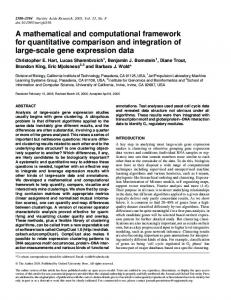
Power Systems Research Group University of Saskatchewan Saskatoon, Canada Abstract--A mathematical framework is presented in this paper for operating reserve assessment based on a hybrid deterministic/probabilistic approach. The approach known as system well-being embeds the conventional deterministic criteria into a probabilistic method. The proposed mathematical framework includes the computational requirements in both spinning and supplemental reserves. Interruptible load is also included in the framework as part of the operating reserve. The impact of ramp-rate limits on economic load dispatch is incorporated in the overall framework. The computational tools required to incorporate factors such as load forecast uncertainty and postponable outages are also presented. Keywords: power system reliability, unit commitment, spinning reserve, operating reserve, well-being approach 1. INTRODUCTION Operating reserve requirements in today’s electric power industry are usually determined using deterministic criteria or rule-of-thumb methods. The essential disadvantage of deterministic criteria is that they do not respond to the many factors that influence the actual risk in the system. Utilization of probabilistic techniques will permit the capture of the random nature of system component and load behavior in a consistent manner. Despite the obvious disadvantages of deterministic approaches, there is considerable reluctance to apply probabilistic techniques to assess spinning reserve requirements [1-3]. This reluctance dictates a need to create a bridge between the deterministic methods and the prevalent probabilistic techniques. This formulation, designated as system well-being, in the form of system health, margin and at risk, can play an important role in providing system operators with a better understanding of operating reliability. In the well-being approach, the probability of the system being in the healthy state together with the conventional risk index can be used as system operating criteria [4-6]. An overall mathematical framework is presented in this paper for determining the reserve requirements based on the well-being approach. The framework includes the computational requirements in both spinning and supplemental reserves. Non-spinning reserves such as rapid start gas turbine units and hot reserve units are assessed using the concepts of area risk curves where the associated lead times play a key role in the analysis. Interruptible load is also included in the framework as part of the operating reserve depends on the time of
interruption [1,7,8]. Once the required amount of operating reserve is determined, the impact of ramp-rate limits on economic load dispatch is incorporated. Inclusion of all these facilities in unit commitment and operating reserve assessment requires different techniques and computational tools. Factors such as load forecast uncertainty and postponable outages are also included in the framework. The presented mathematical modeling is easy to program and there are no restrictions on the size of the system. 2. WELL-BEING MODEL In order to incorporate practical security considerations in operating reserve assessment, the system performance can be divided into operating states classified in terms of the degree to which the adequacy and security constraints are satisfied. The system states, designated as healthy, marginal and at risk are shown in Figure 1. Healthy
Marginal
At Risk
Figure 1. Well-being model.
The system operates within the specified limits in both the healthy and marginal states. In the healthy state all the equipment and security constraints are within limits while supplying the total system demand. In this state, there is sufficient reserve margin such that accepted deterministic criterion, such as any single contingency, can be tolerated without violating the limits. In the marginal state, the operating constraints are within limits, but some specific single contingencies will result in a limit being violated due to insufficient reserve margin. The system is, therefore, on the edge of being in trouble in this state. The operating constraints are violated in the risk state and the system may be required to shed load in this state. The probabilities associated with the healthy and risk states can be considered as operating reserve criteria. A contingency enumeration technique is used to calculate the well-being indices, i.e. healthy, marginal and risk state probabilities. For a given contingency, the security constraints must be tested before it is judged to be a successful state (healthy or marginal) or a failed state
14th PSCC, Sevilla, 24-28 June 2002
Session 05, Paper 1, Page 2
(risk). The decision on whether a given successful contingency belongs to the healthy or marginal states cannot be made correctly unless all possible next level outages involving that particular outage are examined. A comprehensive mathematical framework is presented in the following sections for various aspects of operating reserve well-being analysis. 3. GENERATING UNIT AND INTERRUPTIBLE LOAD MODELS Operating reserve can be generally divided into the two classes of unit reserve and system reserve. Unit reserve may be in the form of spinning or stand-by units. Figure 2 shows a modified two-state model [7] used in operating reserve assessment for spinning units. It is assumed that the system lead time is relatively short and therefore the probability of repair occurring during the small lead time is negligible. Under this condition the time dependent probabilities of the operating and failed states for a unit can be approximated by Equations 1 and 2, respectively, at a given delay time of T.
O
λ
(1) (2)
Where λ is the unit failure rate and ORR is the outage replacement rate [7]. The two-state model can further be modified by including postponable outages. In this case the total unit failure rate is reduced by the degree of postponability β. The probability of finding the unit in the failed state at a given time T in the future can be obtained using Equation 3 [7]. P( failed ) ≅ ( λ − βλ )T = ( 1 − β )λT 0 ≤ β ≤ 1 (3) Rapid start and hot reserve units are represented by four and five state models as shown in Figures 3.a and 3.b respectively [9]. The time dependent state probabilities are evaluated using a matrix multiplication technique.
[P( t )] = [P( t0 )][P]m
λ 41
λ 14
m= t0 = tr t0 = th
λ 23
Cold Reserve
λ 25
1 In Service
λ 41
λ 14
λ 51
λ 21 λ 15
2
λ 12
Ready for Service
λ 45
5
λ 52
λ 21 2
1 λ 12
Hot Reserve
(a)
In service
(b)
Figure 3: Four and five state models for rapid start and hot reserve units respectively.
[P( tr )] = [P1( tr )
0 0 P4 ( tr )]
[P( th )] = [P1( th )
(5)
0 0 P4 ( th ) 0 ]
(6)
λ23 P4 ( tr ) = λ21 + λ23
(7)
P1( tr ) = 1 − P4 ( tr )
(8)
λ23 + λ24 λ21 + λ23 + λ24
(9) (10)
The probabilities of finding the rapid start and hot reserve units on outage given that a demand has occurred are given by Equations 11 and 12 respectively. The unit availabilities are calculated using the complementary values of Equations 11 and 12. P( Down ) =
P3 ( t ) + P4 ( t ) P1 ( t ) + P3 ( t ) + P4 ( t )
(11)
P( Down ) =
P3 ( t ) + P4 ( t ) + P5 ( t ) P1( t ) + P3 ( t ) + P4 ( t ) + P5 ( t )
(12)
Interruptible load can be modeled as an equivalent generating unit with zero failure rate or considered as a load variation as shown in Figures 4 and 5 respectively where τ is the load interruption time. In this paper, the load variation model is used for the purpose of computational analysis. MW
spinning capacity
C+IL C
(4)
total load
L
Where
[P( t )] = [P( t0 )] = [P] =
λ 24
λ 42
λ 32
4
3
4
P1( th ) = 1 − P4 ( th )
F
Figure 2. Two-state model of a generating unit used in operating reserve evaluation.
P( failed ) ≅ λT = ORR P( operating ) ≅ 1 − λT
λ 34
λ 23
Failed
λ 34
Failed
3
P4 ( th ) =
Failed
Operating
Fail to Take up Load
Fail to Start
vector of state probabilities at time t, vector of initial probabilities, stochastic transitional probability matrix, number of time steps used in the discretization process. lead time of rapid start units lead time of hot reserve units
The vector of initial probabilities for the rapid start and hot reserve units are given in Equations 5 and 6 respectively.
τ
0
T
time
Figure 4. Equivalent unit approach model for interruptible load. MW
spinning capacity
C
total load
L
firm load
L-IL 0
τ
T
time
Figure 5. Load variation approach model for interruptible load.
14th PSCC, Sevilla, 24-28 June 2002
4. MATHEMATICAL EXPRESSIONS
Session 05, Paper 1, Page 3
Pr 5
risk calculated for the
on-line units
NO
+
NRS rapid start units and load demand of ( L - IL ) at time th ,
The symbols used in this section are defined as follows:
risk calculated for the NO on-line units + NRS
Pr 6
Ph , Pm , Pr
specified healthy and risk state probabilities, actual healthy, marginal and risk state
Pr7
P1h , P1m , P1r
probabilities using the area risk curve F2 ( R ) , calculated healthy, marginal and risk state probabilities considering only spinning capacity (area risk F1( R ) ),
L τ IL ta
system load demand, interruption time of interruptible load, interruptible load, lead time of additional generating units in the system,
t r , th
lead time of rapid start and hot reserve units, Standard deviation in the normal distribution,
SPh , SPr
Ri , Rii , Riii , Riv NRS , NHR
partial risks number of rapid start and hot reserve units,
marginal and risk state Ph ( i ), Pm ( i ), Pr ( i ) healthy, probabilities respectively, associated with the ith step load level in the normal distribution, k partial risks associated with the ith step load Rik , Riik , Riii , Rivk
rapid start units + NHR hot reserve units and load demand of ( L - IL ) at time th , risk calculated for the NO on-line units + NRS rapid start units + NHR hot reserve units and load demand of ( L - IL ) at time ta ,
SD Al ( i )
RPh , RPm , R Pr
level in the normal distribution, response healthy, marginal and risk state
Lk
probability of the load being at the ith class interval in the normal distribution, number of steps in the normal distribution (an integer odd number) load associated with the kth class interval in the
RPhk , RPmk , R Prk
probabilities, response healthy, marginal and risk state
R Sk
normal distribution total available response associated with the kth class
SOC k
interval in the normal distribution, total system operating cost associated with the kth
MT
class interval in the normal distribution, margin time,
SRPh ,SRPr F1( R ) F2 ( R ) Fi Ai , Bi ,Ci
∆L ∆F ARESc Prk
k probabilities given that CAPrsu response is available from rapid start units, specified response healthy and risk state probabilities, area risk function considering only spinning capacity, area risk function including rapid start, hot reserve and interruptible load, operating cost of the ith committed unit,
RRM TR S
required regulating margin,
TSOC LCi
total system operating cost,
cost parameters of the ith committed unit, incremental load, incremental cost,
SRCi
spinning reserve capacity of unit i,
i RCsru
RESsru
response capability of the ith spinning unit, response from spinning units,
total available response at contingency c,
RESrsu
response from rapid start units,
RESint
response from interruptible loads,
i RESsru
response from the ith spinning unit,
i RESrsu
response from the ith rapid start unit ,
GRSi
maximum capacity of the ith rapid start unit,
maximum capacity of unit i,
i RRsru
response rate of the ith spinning unit,
risk calculated for the on-line units NO
i RRrsu
response rate of the ith rapid start unit ,
and load demand of L at time tr ,
λisru
failure rate of the ith spinning units,
risk calculated for the NO on-line units +
NC
number of capacity states in the COPT,
j CAPsru
response capacity of the jth
j PCsru
associated with the on-line spinning units, probability of the jth capacity state in the COPT
th
risk of k
period in the area risk curve
F2 ( R ) , TDr NO Gi Pr 1 Pr 2
s
total decreased risk due to the inclusion of stand-by units and interruptible loads, number of on-line committed units,
NRS rapid start units and load demand of L at time tr , Pr 3
risk calculated for the NO on-line units +
Pr 4
NRS rapid start units and load demand of L at time τ , risk calculated for the NO on-line units + NRS rapid start units and load demand of ( L - IL ) at time τ ,
total available response at the margin time of MT, loading capacity of unit i,
state in the COPT
associated with the on-line spinning units, i RCrsu j CAPrsu
response capability of the i th rapid start unit within the margin time of MT, response capacity of the jth state in the COPT associated with rapid start units,
14th PSCC, Sevilla, 24-28 June 2002
Session 05, Paper 1, Page 4
j PCrsu
probability associated with the jth response capacity
Pc
state in the COPT of rapid start units, probability of contingency c,
t
Riv = ∫ a F2 ( R )dt = Pr7 − Pr 6
(18)
th
The unit commitment scheduling is started by committing a number of units starting with the most economic unit. The initial number of committed units is therefore the minimum number of units required to satisfy Equation 13. NO
∑ Gi > L
(13)
i =1
The upper curve in Figure 6 shows a possible area risk curve for a system with no stand-by units and interruptible load. This area risk curve represents the behavior of the system when only spinning and synchronized units (on-line units) are considered in the reserve calculations. A typical area risk curve for a system with rapid start, hot reserve units and interruptible load is shown in the lower curve of Figure 6. F1 ( R )
It is assumed that the system is not in trouble at the decision time of t=0 and therefore Pr 0 is zero. In addition, it is also assumed that there is enough capacity available after the system lead time ta such that the risk after this time is negligible. The calculated system risk is compared with the specified risk as shown below. Pr ≤ SPr
(19)
If Equation 19 is not satisfied, an additional unit is added to the already on-line committed units and the above procedure is continued until the system risk is satisfied. Once the system risk is satisfied, the healthy and marginal state probabilities are calculated as follows. t
t
0
0
TDr = ∫ a F1( R )dt − ∫ a F2 ( R )dt
(20)
TDr = P1r − Pr
(21)
P1r is determined from a COPT made of NO on-line committed units. The COPT represented in a descending order is shown in Table 1. Each unit is represented by the two-state model shown in Figure 2. The failed and operating state probabilities are calculated as follows. P( failed ) ≅ λirsu × ta P( operating ) ≅
0
ta
time
F2 ( R ) rapid start units are available
P1r =
hot reserve units are available
1 2
∑ Pi × Qi L < Ci
3 4
5 6
7
The system risk can be calculated by simulating all possible contingencies. Evaluation can require a considerable computation time specially for systems with a large number of committed units. In order to decrease the computational time the partial system risk at each period is determined using a capacity outage probability table (COPT) [7]. Using the initial number of committed units the system risk is calculated in the presence of rapid start units, interruptible load and hot reserve units. Pr = Ri + Rii + Riii + Riv tr
F2 ( R )dt = Pr 1 − Pr 0
τ
Rii = ∫ F2 ( R )dt = Pr 3 − Pr 2
(14) (15)
Riii =
th
∫τ
F2 ( R )dt = Pr 5 − Pr 4
P1
C2
P2
. .
. .
0
P2
NO
The healthy state probability, P1h , cannot be calculated using the COPT and is determined using a contingency enumeration technique. For a given contingency c it is assumed that m1 set of units are in service and m 2 set of units are out of service. m1 + m2 = NO
(26)
m1
m2
i =1
j =1
j Pc = ∏ ( 1 − λisru × ta )∏ ( λsru × ta ) m1
( ∑ Gi ) − Gk > L i =1
(∑ Pc
(16)
P1h =
(17)
P1m = 1 − P1h − P1r
tr
Individual probability
1
C
Riv
ta time τ th tr Figure 6. Area risk curves with and without stand-by units and interruptible loads.
∫0
(25)
L ≥ Ci
0
Ri =
(24)
i =1
Capacity in service Riii
(23)
Table 1. COPT of the NO on-line spinning units.
additional units are available
Rii
× ta
NO
0 if Qi = 1 if
IL is interrupted
Ri
2
(22)
1 − λirsu
(27)
k ∈ m1 set of units
if Equation 28 is satisfied
)
(28) (29) (30)
14th PSCC, Sevilla, 24-28 June 2002
Session 05, Paper 1, Page 5
Comparing the two area risk curves F1( R ) and F2 ( R ) : Pr = 1 − P1h − P1m − TDr
(31)
Pr = 1 − P1h − P1m − TDr + (P1h + P1m )TDr −
(P1h + P1m )TDr
(32)
Pr = 1 − [P1h (1 + TDr ) + P1r × TDr ] − [P1m (1 + TDr )]
(33)
Pr = 1 − Ph − Pm
(34)
Ph = P1h (1 + TDr ) + P1r × TDr
(35)
Pm = P1m (1 + TDr )
(36) If the unit commitment criterion is to satisfy a single risk criterion, the procedure is stopped here. Otherwise the health criterion is checked as shown below: (37) Ph ≥ SPh If the health criterion is not satisfied, one more unit is committed in addition to the already on-line committed units and the procedure is continued until the criterion is satisfied. Load forecast uncertainty can be included in the wellbeing analysis as some deviation always exists between the forecast and the actual loads. The uncertainty is described by a normal distribution in which the distribution mean is the forecast load L and the standard deviation is obtained from previous forecasts [7]. The normal distribution can be divided into class intervals as shown in Figure 7 whose number depends upon the accuracy required. The area of each class represents the probability of the load being at the class interval mid value. The operating state probabilities for each load level Lk are first calculated and then weighted by the probability of the load being in each level
s/2 Ph ( i ) × Al ( i ) ∑ i = −s / 2 s/2 Pm = Pm ( i ) × Al ( i ) ∑ i = −s / 2 s/2 ∑ Ph ( i ) × Al ( i ) ≥ SPh i = − s / 2 Ph =
(42) (43) (44)
The healthy, marginal and risk state probabilities associated with each load level are used to compute the overall health, margin and risk indices. The overall values are compared with the criterion values. Once the number of committed units are determined for a specified unit commitment criterion, the next step is to determine the well-being indices with respect to the response capability of the generating system. The actual operating ranges of all the committed units are restricted by their ramp rate characteristics [10-11]. The total response output can be provided by spinning units, rapid start units and interruptible loads. Rapid start units and interruptible loads can contribute to the response output if Equations 45 and 46 are satisfied. tr < MT
(45)
τ ≤ MT
(46)
TR = Rsru + Rrsu + Rint
(47)
Gi
Gi SRCi = RCi
LCi
SRCi
RCi
LCi
0
(a)
MT
0
MT
(b) Gi
Al ( 0 ) Al ( −1 )
SRCi RCi
Al ( 1 )
Al ( − s / 2 )
LCi
Al ( s / 2 )
0
(c)
MT
Figure 8. Response characteristics of spinning units. -S/2
-1
0
1
S/2
Number of standard deviation from the mean
Figure 7. Class intervals of normal distribution. .
Lk = L( 1 + SD × k )
s s k = - ,....,0 ,....,+ 2 2
k Pr ( k ) = Rik + Riik + Riii + Rivk
s/2 Pr ( i ) × Al ( i ) ∑ i = −s / 2 s/2 ∑ Pr ( i ) × Al ( i ) ≤ SPr i = − s / 2
Pr =
(38) (39) (40) (41)
The response characteristics of the spinning units can be categorized into three classes as shown in Figure 8. The three classes are defined as follow: SRCi = RCi SRCi < RCi SRC > RC i i
Figure 8.a Figure 8.b Figure 8.c
Group I Group II Group III
(48)
The response characteristic of a rapid start unit is represented in Figure 9. The overall system response characteristic is shown in Figure 10, in which the total response in the system is provided by on-line spinning units, rapid start units and interruptible load. Similar to the case of unit commitment, the response risk is first determined for each load dispatch using a capacity outage probability table (COPT). The COPT is obtained
14th PSCC, Sevilla, 24-28 June 2002
Session 05, Paper 1, Page 6
by combining all the spinning committed units. The capacity associated with each unit is the available response capacity of that unit.
associated with a rapid start unit at the margin time of MT is calculated as follows.
(
i i RESrsu = Min GRSi , RCrsu
)
(53)
where GRSi
i i RCrsu = RRrsu × (MT − tr )
GRSi
(54) NRS
i RES rsu
0
tr
i RESrsu
0
MT
tr
MT
Figure 9. Response characteristics of rapid start units. Res(t)
response due to interruptible load
where The total number of states in the COPT is 2 NRS is the total number of rapid start units. Both COPTs are arranged in descending order, i.e. j j +1 CAPsru > CAPsru
for
j = 1,2 ,..., NC − 1
(55)
j j +1 CAPrsu > CAPrsu
for
j = 1,2 ,...,2 NRS − 1
(56)
Table 3. COPT of the available response of the rapid start gas turbine units.
response by rapid start units
Response capacity
Individual probability
1 CAPrsu
1 PCrsu
2 CAPrsu
2 PCrsu
. .
. .
response by spinning units t
0
r
τ
MT
0
time
Figure 10. Overall system response characteristic.
{
i i RESsru = Min (Gi − LCi ), RCsru
}
(49)
The contribution of rapid start gas turbine units to response capability is considered using the conditional probability approach. RPr =
where i i RCsru = RRsru × MT
(50)
Each unit is represented by a two-state model where the failed and operating state probabilities are calculated as follows. P( failed ) ≅
λisru
P( operating ) ≅
× MT
1 − λisru
(51) × MT
(52) The COPT is represented by an equivalent multi-state unit model as shown in Table 2. In this case, the number of units contributing to create the COPT is not necessarily NO as the response from some of the units which are operating at their maximum capacity is zero. Table 2. COPT of the available response of the on-line spinning units.
Response capacity
Individual probability
1 CAPsru
1 PCsru
2 CAPsru
2 PCsru
. .
. .
0
NC PCsru
The available response from rapid start gas turbine units at the margin time of MT can also be represented in the form of a COPT as shown in Table 2. The capacity associated with each unit is the available response capacity of a rapid start unit at the margin time of MT. The associated probability at MT is calculated using the complement of Equation 11. The available response
NRS
2 PCrsu
2 NRS
k ∑ RPrk × PCrsu
(57)
k =1
for the kth state of the rapid start units COPT(Table 3), the total available response is equal to: k CAPrsu + RESint + response of spinning units
RPrk is found from Table 2 as shown below. RPrk =
NC
i × Qi ∑ PCsru
(58)
i =1
0 if Qi = 1 if
i k + RESint + CAPrsu RRM < CAPsru i k + RESint + CAPrsu RRM ≥ CAPsru
(59)
The calculated response risk is compared with the specified response risk as shown below. RPr ≤ SRPr
(60)
If Equation 60 is not satisfied, the load dispatch must be readjusted to increase the total response from the on-line committed units. This is done by taking away an incremental load from a unit in Group II whose incremental running cost is the highest and giving to a unit in Group III whose incremental running cost is the lowest. If the cost model is defined as Equation 61, the incremental running cost of unit k for an increasing load of ∆L and that of unit j for a decreasing load of ∆L are calculated using Equations 62 and 63 respectively. Fi = Ai + Bi × LCi + Ci × LCi2 (61) (62) ∆Fk = ∆L [ Bk + Ck ( 2 LCk + ∆L )] (63) ∆F j = ∆L [ B j + C j ( 2 LC j − ∆L )]
14th PSCC, Sevilla, 24-28 June 2002
Session 05, Paper 1, Page 7
The total running cost increases by ( ∆Fk − ∆F j ) .
system response are given by:
The response risk is calculated after each reloading step and is continued until Equation 59 is satisfied. Once the response risk criterion is satisfied, the next step is to calculate the response healthy and marginal state probabilities as follows.
TSOC =
RPh =
2 NRS
k ∑ RPhk × PCrsu
(64)
k =1
RPhk
is calculated using a contingency enumeration technique. For a given contingency the on-line committed units are arranged into two sets, where in set 1 m1 units are in service and in set 2, m2 units are on outage. The probability associated with the contingency c, Pc , is calculated using Equation 2. m1 + m2 = NO
(65)
m1
m2
i =1
j =1
j Pc = ∏ ( 1 − λisru × MT )∏ ( λsru × MT ) m1
∑ LCi + ARESc > ( RRM + L )
(66) (67)
i =1
j ARESc − RESsru > LC j
j ∈ m1 set of units
m1 i k ARESc = ∑ RES sru + RESint + CAPrsu i =1
(68) (69)
If both Equations 67 and 68 are satisfied, the contingency lies in the healthy state. By varying m2 from 0 to NO , all possible contingencies are considered. RPhk =
{∑ Pc
}
contingency c belongs to the healthy state
RPm = 1 − RPh − RPr
(70) The calculated response healthy state probability is compared with the specified response health as shown below. RPh ≥ SRPh
(71)
If Equation 71 is satisfied, the final load dispatch is considered as an acceptable and optimum one. The total system operating cost and the expected system response are given by Equations 72 and 74 respectively. TSOC =
NO
∑ Fi
(72)
i =1
TRS = response from spinning units + response from rapid start units + interruptible load TRS =
2 NRS i k k RES + × PCrsu + RESint ∑ sru ∑ CAPrsu i =1 k =1 NO
(73) (74)
If the response criterion is not satisfied, the load dispatch must be readjusted or more unit(s) should be committed to provide additional response. The impact of load forecast uncertainty can also be included in the ramp rate constraint economic load dispatch similar to the unit commitment situation discussed earlier. The expected system operating cost and
s/2
∑ SOC k × Al ( k )
(75)
k =−s / 2
TRS =
s/2
∑ RS k × Al ( k )
(76)
k =− s / 2
Acceptable system operating requires that the system healthy state probabilities are maintained at acceptable levels in both the unit commitment and response analysis while minimizing the system operating cost. 5. CONCLUSION An overall mathematical framework is presented in this paper for determining operating reserve requirements based on the well-being approach. The framework includes the respective mathematical formulations required for both spinning and supplemental reserves. Non-spinning reserves such as rapid start gas turbine units and hot reserve units are assessed using the concept of area risks. Interruptible load is also included in the framework as part of the operating reserve. The mathematical formulations required to incorporate the ramp-rate constraints in economic load dispatch is also presented. The incorporation of load forecast uncertainty and postponable outages are also included in the framework. The mathematical models presented can be extended to operating reserve requirements in interconnected systems. REFERENCES [1]
Nish, J. I. and Millar, N. A., "Generation System Operating Reserve Assessment Practices used by Canadian Utilities", Electrical Association, Power System Planning and Operation Section, Spring Meeting 1984. [2] Final Report, "Composite-System Reliability Evaluation: Phase 1 - Scoping Study ", Tech. report EPRI EL-5290, Project 2581-1, December 1987. [3] NERC Operating Manual, 1995. [4] Billinton, R., Fotuhi-Firuzabad, M., “A Basic Framework For Generating System Operating Health Analysis”, IEEE Transactions on Power Systems, Vol. 9, No. 3, pp. 1610-1617, August 1994. [5] Billinton, R., Fotuhi-Firuzabad, M., “Generating System Operating Health Analysis Considering Standby Units, Interruptible Load and Postponable Outages”, IEEE Transactions on Power Systems, Vol. 9, No. 3, pp. 1618-1625, August 1994. [6] Billinton, R. and Khan, E., "A Security Based Approach to Composite Power System Reliability Evaluation", IEEE Transactions on Power Apparatus and Systems, Vol. PWRS-7, No. 1, pp. 65-71, February 1992. [7] Billinton, R. and Allan, R. N., Reliability Evaluation of Power Systems, Plenum Press, 1984. [8] Salehfar, H., Patton, A. D., "A Production Costing Methodology for Evaluation of Direct Load Control", IEEE Transactions on Power Systems, Vol. 6, No. 1, Feb 1991, pp. 278-284. [9] Billinton, R., Jain, A. V., "The Effect of Rapid Start and Hot Reserve Units in Spinning Reserve Studies", IEEE Transaction on Power Apparatus and Systems, Vol. PAS-91, pp. 511-516, 1972. [10] Stadlin, W. O, "Economic Allocation of Regulating Margin", IEEE paper No. 71 TP99-PWR, Nov. 1970. [11] Wang, C.; Shahidehpour, S.M.; “Effects of Ramp-rate Limits on Unit Commitment and Economic Dispatch”, IEEE Transactions on Power Systems , Vol. 8, No. 3, pp. 1341-1450, Aug. 1993.