We present a new model for all solid-state lithium ion batteries that takes into account detailed aspects of ion transport in solid solutions of crystalline metal ...
A Mathematical Model for All Solid-State Lithium Ion Batteries Katharina Becker-Steinberger, Stefan Funken, Manuel Landstorfer und Karsten Urban
Preprint Series: 2009-26
Fakult¨ at fu ¨ r Mathematik und Wirtschaftswissenschaften ¨ ULM UNIVERSITAT
A Mathematical Model for All Solid-State Lithium Ion Batteries K. Becker-Steinberger∗ , S. Funken∗ , M. Landstorfer∗ , and K. Urban∗ ∗
Institute of Numerical Mathematics, University of Ulm, 89081 Ulm, Germany We present a new model for all solid-state lithium ion batteries that takes into account detailed aspects of ion transport in solid solutions of crystalline metal oxides. More precisely, our model describes transient lithium ion flux through a solid electrolyte, the solid–solid interfaces and an intercalation electrode. The diffuse part of the double layer is dynamically described via the Poisson equation, while the Stern layer potential drop is modeled by a Robin boundary condition. Electrochemical reactions on the electrode/electrolyte interface are modeled via non-linear Neumann boundary conditions. After a detailed derivation of the model equations and boundary conditions, numerical results are presented and discussed. 1. Introduction
For a combined solar cell-battery device classical liquid electrolytes are not able to guarantee long-term stability as temperature rises up to 150◦ C on the backside of a solar cell. Switching to solid electrolytes with crystalline structure does not only provide thermal stability, long-term cycling stability and safety benefits, but also an improved diffusivity as temperature rises. A promising crystalline solid electrolyte is Li5+x BaLa2 Ta2 O11.5+0.5x , x ∈ [0, 2] (1) with a lithium ion conductivity of 105 to 5 · 105 [S · cm−1 ]. To gain a better understanding of the limiting processes within the battery cell, a mathematical model which describes the transport of lithium ions in detail, is of great interest. This model has to take into account the flat or non-porous solid electrolyte/electrode interface and the chemical reactions occurring at that interface. Since the interface is quite small compared to porous liquid electrolyte/electrode interfaces, it is important to accurately describe the electrochemical reaction in a mathematical sense. Furthermore, we cannot assume the classical double layer model at the interface, as we have a fixed anion structure which leads to a different ion distribution (2,3) near the interface, as compared to liquid electrolytes. In addition, the desired thin film lithium ion battery cell has an electrode thickness of about 300nm and electrolyte thickness of 200nm. In this case, we cannot assume anymore linear potential drop across the solid electrolyte. Hence, we have to model a solid electrolyte as a Poisson-Nernst-Planck (PNP) equation system which does not assume local electroneutrality nor any classical model for the diffuse part of the double layer. In contrast to classical models for lithium ion batteries (4-6), we explicitly compute the diffuse part of the double layer and model the Stern layer potential drop by a Robin type boundary condition. This allows us to couple electrochemical reactions with the dynamic Stern layer potential drop which are mathematically described as a non-linear Neumann boundary conditions. In Section 2, we explain the model equations for the solid electrolyte and the intercalation cathode, while in Section 3 we give a detailed derivation of the boundary conditions for the electric potential on the solid electrolyte/electrode interface and the lithium ion flux. Numerical results are given and discussed in Section 4, followed by a summary in Section 5.
Schematic 3-D Cell z y
Deflector Anode
x
Electrolyte
Electrolyte
Cathode
Anode
Cathode
Ω1
Ω2
Model Geometry
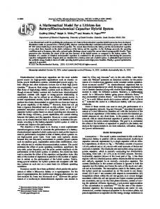
Figure 1: Model reduction from a whole 3-D battery cell to a battery cross section. 2. Model Assumptions and Transport Equations Before we derive the model equations and the related boundary conditions, we collect our model assumptions. 1. The battery cell is reduced to a 1-D geometry which is motivated by the assumption of isotropic transport properties in y- and z-direction, see Figure 1. 2. We assume perfect planar interfaces between the solid electrolyte and the electrodes. In our 1-D geometry, this assumption complies to a pointwise coupling between the electrode and electrolyte while in a full 3-D geometry it refers to a 2-D interface. Even if the interface is not perfectly planar, this assumption is valid for solid electrolytes. This can be seen by considering mapping strategies from rough 2-D interfaces to a planar interface which will be discussed in a forthcoming paper. 3. (Electro-) chemical reactions only occur at the planar interfaces, since we assumed no porous electrodes and not any phase transformation yet. 4. In the solid electrolyte, we do not take into account repulsive ion-ion interaction which could be operative in regions where the ion concentration is high. However, this is part of our current research and results will be published in soon elsewhere. This assumption yields to a constant diffusion coefficient for the lithium ions in the solid electrolyte. 5. Further on, we do not explicitly model any electron transport. Hence, we assume that electrons are always and instantaneously available. This assumption could be crucial for semiconductors, but follows classical models for battery systems. 6. Particle diffusion within the electrodes only occurs as interior diffusion, while the process of intercalation only happens at the planar interface. This could be thought of as perfect mono-crystalline structures. We do not take into account surface diffusion. 7. We consider the potentiostatic case. 8. Potential variations as function of status of charge (SOC) were not yet taken into account. 9. The anode is a lithium foil without any diffusion processes. Thus, we only model diffusion processes within the solid electrolyte and the intercalation cathode. 10. We neglect elastic effects of intercalation on the the reacting phases. Especially in an
all solid-state battery, intercalation induced stress in the electrodes plays an important role in terms of long time cycling stability. This is part of our current research and results will be published in soon elsewhere. The considered battery cell consists of a lithium foil anode, a solid electrolyte, and an intercalation cathode. Thus, the battery cell cross section Ω = ∪i Ωi , i = 1, 2, can be described as union of two one-dimensional segments of length Li , i = 1, 2. Here, Ω1 corresponds to the solid electrolyte and Ω2 to the positive electrode of the lithium ion battery (compare Figure 1). To describe macroscopic phenomena occourring during battery discharge appropriately, equations specifying mass transfer in both phases and charge distribution in the electrolyte are needed. The continuum fields representing the state of the solution in the electrolyte are + the lithium ion concentration CLi (X1 ,t), the electrostatic potential Φ(X1 ,t) and the lithium concentration in the electrode CLi (X2 ,t). The derivation of the equations for the solid electrolyte is followed by those for the cathode. In each region species mass balance holds, i.e., ∂ Ji ∂Ci =− , ∂t ∂ Xj
j = 1, if i = Li+ , else j = 2,
[1]
thus modeling mass transfer for species i reduces to the description of the particle flux Ji . Transport equations for the solid electrolyte Because charged particles move due to diffusion and electromigration processes, we assume a Nernst-Planck flux (7-10) in the electrolyte � � ∂CLi+ ∂Φ JLi+ = − DLi+ + µLi+ CLi+ , [2] ∂ X1 ∂ X1 where the diffusion coefficient DLi+ and the mobility µLi+ are assumed to be constant. With the Nernst-Einstein relation, the mobility of a species i can be expressed in terms of its diffusivity µi = zi FDi /RT . Here, R denotes the universal gas constant, T the absolute temperature and F the Faraday’s constant. Since lithium has a single valance electron, the charge number after oxidation is zLi+ = 1. Hence, we omit the charge number in the following. Substituting the universal Nernst-Einstein relation into [2] and inserting the Nernst-Planck flux in the continuity equation [1], we obtain the following transport equation for lithium ions in the solid electrolyte � � ∂ 2CLi+ FDLi+ ∂ ∂Φ ∂CLi+ = DLi+ + CLi+ . [3] ∂t RT ∂ X1 ∂ X1 ∂ X12 Charged particles migrate due to an electric field which is related to the electric potential by the Gauss law E = −∂X1 Φ. Furthermore, it can be shown that this also holds for time dependent electric fields at the time scales under consideration, since in this case magnetic effects are negligible (7). The electrostatic potential is related to the volume charge density via the Poisson’s equation −εb
∂ 2Φ =ρ ∂ X12
[4]
where εb is the constant permittivity of the bulk solvent and ρ is the volume charge density. The charge density is a function of the concentrations of the charged particles and thus a function of space and time, ρ(X1 ,t) = F · (CLi+ (X1 ,t) − CA ). In the case of a solid electrolyte with a fixed anion structure like an anion jelly, ρ is only dependent on the lithium ion concentration while the anion concentration CA is constant (8). Due to the fact that in the bulk electrolyte anion and cation concentrations are equal, the resulting electric field is constant. In particular the diffuse double layer is explicitly calculated. Transport equations for the intercalation cathode Lithium ion flux of intercalated lithium is described via Fick’s first law of diffusion which states that the particle flux is proportional to the negative concentration gradient (4-6). Conservation of mass [1] and the assumption of a constant diffusion coefficient lead to ∂CLi ∂ 2CLi = DLi . ∂t ∂ X22
[5]
Although electrons for intercalated lithium are dislocated, we think of intercalated lithium ions as formally neutral particles. Thus equation [5] can also be interpreted as special case of [2] with zLi = 0, i.e., without elecromigration. Combining [3 - 5] results in a non-linear system of drift-diffusion partial differential equations (PDE) for the unknown CLi ,CLi+ and Φ, where the non-linearity arises from to the convective term CLi+ ∂X Φ in the Nernst-Planck equation [3]. To obtain a non-dimensional system, we scale all quantities appropriately. The resulting dimensionless variables are xi =
Xi , i = 1, 2, Li
τ = δt,
c=
CLi+ , bulk CLi +
ρ=
CLi max , CLi
ϕ=
FΦ . RT
[6]
Here we scale each length according to the length of the corresponding component, potential to the thermal voltage F/RT and concentrations to maximum concentrations or bulk concentration. We obtain dimensionless unknowns c(x1 , τ), ρ(x2 , τ) and ϕ(x1 , τ). The equation system [3 - 5] becomes � � ∂2 ∂ ∂ ∂ L1 δ c(x1 , τ) = DLi+ 2 c(x1 , τ) + DLi+ c(x1 , τ) ϕ(x1 , τ) , [7] ∂τ ∂ x1 ∂ x1 ∂ x1 0 = ε2
1 ∂2 ϕ(x , τ) + (c(x1 , τ) − cA ), 1 2 ∂ x12
∂ ∂2 L2 δ ρ(x2 , τ) = DLi 2 ρ(x2 , τ), ∂τ ∂ x2 with ε := λD /L1 and λD :=
[8] [9]
q bulk . εb RT /2F 2CLi +
3. Boundary conditions for the potential and the concentrations The description of the boundary phenomena at the electrochemical interface, i.e., the double layer and the electrochemical reactions, is mathematically formulated by Robin- and
Neumann boundary conditions. First of all, we derive the boundary condition for the electric potential at the interface followed by the derivation of the lithium flux boundary condition using classical first order redox reactions and transition state theory. In particular, the lithium flux boundary condition is a coupling boundary condition connecting the mass transport between the two phases Ω1 and Ω2 . Robin boundary conditions for the electrical potential A closer look to the solid electrolyte/electrode interface, where both regions are treated as a continuum mechanical model, yields to the unknown potential drop ∆ΦS . In general, the potential drop can be calculated via Φ(XR ) = Φ0 − ∆ΦS (compare Figure 2). This potential drop can be modeled as the potential drop across an ideal plate capacitor with capacity CˆS under the following assumptions: • The relative permittivity εr of the dielectric is constant. Note that this is not true in general, as the potential drop of 1 − 2V occur at 1 − 2 Angstroms, resulting in an electric field of orders of 109V /m. • Intercalation and adsorption of the lithium ions does not influence the capacity of the plate capacitor model. With a given capacity CˆS and the capacity per unit area CS of the Stern layer it follows that Q 1 CˆS = = Aε0 εr E, ∆ΦS ∆ΦS
[10]
∂Φ A 1 ∂ Φ ε0 εr = − ε0 εr ∂ X1 CS ∂ X1 X1 =XR CˆS
[11]
and thus ∆ΦS = −
by using Gauss’ theorem E = −∂X1 Φ. Here, Q denotes the charge on the surface area A, ε0 the vacuum permittivity and XR = {0, L1 } the boundary points of the electrolyte in the 1-D model. This results in the following Robin boundary condition (7, 9-11) (for the anode side) ∂ Φ CS CS + = Φ Φ0 . ∂ n X1 =0 ε0 εr X1 =0 ε0 εr
[12]
Note that, we arbitrarily set the electric potential Φ0 on the cathode side to 0 and hence get ∂ Φ CS + Φ = 0. ∂ n X1 =L1 ε0 εr X1 =L1
[13]
The boundary points are denoted with an index R to emphasise that at these points a Robin boundary condition is applied. With these boundary conditions, the model is able to describe the Stern Layer potential drop and the diffuse part of the double layer dynamically and concentration dependent. Furthermore, the potential drop across the Stern layer (12) accelerates the chemical reactions, and not the whole potential drop across the double layer.
! E solid bulk material
Φ0 ∆ΦS
Φ(X1 )
Stern layer
X1 = 0
Figure 2: Solid electrolyte/electrode interface model. Φ0 is the outer electric potential of the solid bulk material, Φ(XR ) is the electric potential right behind the Stern layer. ∆ΦS is the unknown potential drop across the Stern Layer. Neumann boundary conditions for the concentration We start by a general first order redox reaction A B. The classical mathematical description of a first order redox reaction is ∂CA = −k f CA + kbCB | {z } |{z} ∂t A→B
[14]
B→A
with concentrations CA (X,t),CB (X,t) for species A, B, respectively. The reaction rate coefficients k f , kb for forward and backward reactions are calculated via transition state theory. Therefore, the reaction rate coefficient ki can be expressed as ! −∆G‡i kB T ki = exp [15] h RT with Gibbs free energy of activation ∆G‡i for reaction i, Bolzmann constant kB and Planck constant h. Electrochemical reactions are accelerated by the electric potential difference between the two phases, i.e., between the surface of the electrode and the surface of the solid electrolyte. Hence, the energy barrier of the forward reaction is declined by α∆ΦS , while for the backward reaction raised by (1 − α)∆ΦS . Here, α denotes the dimensionsless symmetry factor of the reduction reaction. All parameters except the dependent variables are included in the new pre-exponential factors kˆ f , kˆ b . This leads to the expression ∂ CA (X,t) = −kˆ f CA (X,t)eα∆ΦS (X,t) + kˆ bCB (X,t)e−(1−α)∆ΦS (X,t) . ∂t eq
[16] eq
With η = ∆ΦS − ∆ΦS this is the classical Butler Volmer equation (5). Here, ∆ΦS denotes the equilibrium Stern layer potential drop determined by from the solution of the stationary problem [21 - 27].
Energy ∆G‡f ∆G‡0 f
∆G‡b
α
Reaction coordinate
∆ΦS
Figure 3: Reaction energy barriers for the forward and backward reaction with an additional electrical potential difference between the two reacting phases. Here, ∆G‡0 f is the free energy of activation for the forward reaction with an electric potential drop, while ∆G‡f is the reduced energy barrier, due to the electrical potential difference, for the forward reaction. To relate the outward flux of lithium ions to the surface reaction occurring on the planar interfaces, the surface concentration c˜ is defined. Here, this is done by evaluating the concentration field on the boundary and multiplying by the Van der Waals diameter of the ion dV which is a volume strip of thickness dV , � � mol . [17] c˜ := c(X) x∈∂ Ω dV m2 The whole framework described above for chemical reactions can directly be adapted to surface reactions. This leads to the expression ∂ c˜A = −k f c˜A + kb c˜B . ∂t
[18]
Looking closer at the outward flux of species A through a surface ΓA , it holds that nJA = −∂t c˜A with the outward normal unit vector n of the surface. Taking further the potential dependence of the reaction rate coefficients into account, this leads to the following expression (for the surface ΓA = Ω1 ∩ Ω2 ): nJA = k f c˜A − kb c˜B = k f dV cA ∂ Ω − kb dV cB ∂ Ω 1 2 h i h i α∆ΦS −(1−α)∆ΦS ˆ ˆ = k f dV cA e − kb dV cB e . [19] ∂Ω ∂Ω 1
2
This non-linear Neumann boundary condition also describes the inward flux of species B because of mass conservation. Thus, JB on the reaction boundary ΓB = ΓA = Ω1 ∩ Ω2 in the direction of the negative outward union normal of Ω2 equals this non-linear Neuman boundary condition. Clearly it holds that nJA = −nJB .
[20]
It is also obvious that this argumentation is also true for the anode/solid electrolyte interface and leads to the missing boundary condition for the lithium ion flux at the other boundary
Species A
Surface Reaction
Species B
Figure 4: The outward flux JA in normal direction of species A through a surface ΓA is related to the surface reaction occurring on that surface. Since there is mass conservation, the outward flux JA corresponds to the inward flux JB . vertex of Ω1 for our 1-D case. For the outward flux of intercalated lithium ions, it is natural to assume isolation at the boundary next to the deflector. Hence, we derived all required boundary conditions, leading to a fully-coupled nonlinear PDE-system for lithium ion concentrations and electric potential in the electrolyte and intercalated lithium inside the electrode. The fully non-dimensional system is given in the Appendix. 4. Numerical Results The numerical realization of the time dependent discharge of an all solid-state lithium ion battery has been performed using COMSOL Multiphysics which is a finite element discretization software. Initial Potential and Concentration Distribution across the Solid Elektrolyte 3
Paramter Setting:
Potential Drop ∆Φ S
80
ε 1 = 1.00e+02 L 1 = 1.00e-07 D 1 = 1.00e-13 λ D = 6.23e-11 λ D = (εε 1 RT /2F 2 c bLui l k) 1/ 2
2.5
ϕ
1.5
40
c+ Li
60
2
1
Bulk Li + concentration: ulk cB =3.0e+04 [mol /m 3 ] Li Max. Li + concentration: ax cM =2.6e+06 [mol /m 3 ] Li
20
0.5
∆Φ S
0 0
0.1
0.2
0.3
0.4
0.5
x1
0.6
0.7
0.8
0.9
1
0
!1 0
cdx = c A
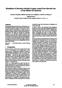
Figure 5: Computed initial condition of the electric potential Φ0 (dashed line) and c0 (solid line). The Stern layer potential drop ∆ΦS is marked by an arrow. Each component Ωi , i = 1, 2, was modeled as a separate geometry and the equations of the dimensionless PDE system [7 - 9] were entered in the ‘PDE General Form” application mode on the appropriate geometry, respectively. The results visualized below were computed by scripting COMSOL with MATLAB. We applied non-uniform quadratic Lagrange-Elements, with 1554 Elements in the electrolyte and 154 in the cathode. Each grid is applied on the non-dimensional domain, i.e., on [0, 1]. The reasons for choosing a non-uniform Finite Element mesh are the different length scales of phenomena. In the
double layer, drift processes, are dominating, mass and therfore charge is varying by a high order of magnitude. We consider an initially fully charged battery cell. For the transient simulation of discharge, an initial condition representing the potential distribution in the electrolyte of a fully charged battery cell is needed. In a mathematical sense, this is equivalent to determine a stationary solution of the coupled PDE system in the electrolyte with homogeneous Neumann boundary conditions for the mass transfer, i.e., with equilibrium chemical reactions at the flat interfaces. Steady state is characterized by ∂τ c = 0, i.e., no variation in time τ. To solve the (nondimensional) stationary system in the electrolyte � � ∂ ∂ ∂2 0 = DLi+ c(·, τ) + DLi+ c(·, τ) ϕ(·, τ) , [21] ∂ x1 ∂ x1 ∂ x1 1 ∂2 ϕ(·, τ) + (c(·, τ) − cA ), [22] 0 = ε2 ∂ x1 2 with isolation and potentiostatic boundary conditions (following (13) define the effective thickness of the compact part of the double layer λs := ε0 εr /Cs and set γ := λS /λD ) DLi+
∂ ∂ c(x1 , τ) + DLi+ c(x1 , τ) ϕ(x1 , τ) = 0, on x1 ∈ {0, 1}, ∂ x1 ∂ x1 ∂ 1 ϕ(0, τ) + ϕ(0, τ) = ϕ0 , ∂ x1 γε ∂ 1 ϕ(1, τ) + ϕ(1, τ) = 0, ∂ x1 γε
[23] [24] [25]
an additional weak constraint is required (10) Z 1 0
c(x1 ) dx1 = cA .
[26]
This integral constraint is not needed when solving the time-dependent problem, since the total number of lithium ions is set by the initial conditions for the concentrations. The integral constraint reflects that in a solid electrolyte the overall amount of the mobile charge carrier species should be equal to the fixed one. From a mathematical point of view the constraint is needed to ensure well-posedness of the stationary system. Figure 5 displays the initial potential distribution across the solid electrolyte including the diffuse part of the double layer (dashed line), the potential drop in the Stern layer (solid labeled line) and the concentration field computed with a constant diffusion coefficient for lithium ions. Figure 6 is just a close-up view to emphasize that the impression of nonsmoothness in Figure 5 is caused by the illustration, i.e., by the scale. As there is no repulsive ion-ion interaction, the lithium concentration on the boundary rises to about 80 times the amount of the bulk concentration. This is still a critical point in our model. The bulk lithium ion concentration of the solid electrolyte is 3.0e + 04[mol/m] for Li5+x BaLa2 Ta2 O11.5+0.5x , x ∈ [0, 2]. Furthermore, the Debey screening length λD displayed here is not the classical Debey-length, but shifting the pre-factors of the Poisson equation in the same way as it is done for liquids, it is equal to what is usually called the
Initial Potential and Concentration Distribution across the Solid Elektrolyte
Paramter Setting: ε 1 = 1.00e+02 L 1 = 1.00e-07 D 1 = 1.00e-13 λ D = 6.23e-11 λ D = (εε 1 RT /2F 2 c bLui l k) 1/ 2
0.5
c+ Li
ϕ
20
Bulk Li + concentration: ulk cB =3.0e+04 [mol /m 3 ] Li Max. Li + concentration: ax cM =2.6e+06 [mol /m 3 ] Li !1
0 0
0.01
0.02
0.03
0.04
0.05
x1
0.06
0.07
0.08
0.09
0
0 0.1
cdx = c A
Figure 6: Detailed view of the potential and concentration distribution near the electrode/solid electrolyte interface. Debey-length. Also note that the bulk concentration is set to 1 and the diffuse part of the double layer is about 1nm, due to the high lithium ion concentration. The simulation result for the transient behavior of an all solid-state lithium ion battery is shown in Figure 7. Note that in the model the chemical reaction is only accelerated due to the Stern layer potential drop in contrast of taking the whole double layer potential drop into account. Together with the assumption of planar interfaces and a non-porous intercalation electrode, this yields to slower chemical reactions compared to models for classical liquid electrolyte batteries (4 - 6). The parameter setting box in Figure 7 includes the total amount of intercalated lithium, i.e., the integral over the concentration of the intercalated lithium. Potential and Concentration Distribution across the Solid Elektrolyte 3
3
Potential Drop ∆Φ S
2.5
2.5
Concentration of Intercalated Lithium inside the Electrode
1
ε 1 = 1.00e+02 L 1 = 1.00e-05 D 1 = 1.00e-12 λ D = 6.23e-11 b u l k 1/ 2 λ D = (εε 1 RT /2F 2 c L i )
0.8
2
2
0.4
Bulk Li + concentration: ulk cB =3.0e+04 [mol /m 3 ] Li Max. Li + concentration: M ax c L i =7.8e+04 [mol /m 3 ]
0.2
!1
ρ
c+ Li
ϕ
0.6 1.5
1.5
1
1
0.5
0.5
0 ∆Φ S
0 0
0.2
0.4
x1
0.6
0.8
1
Paramter Setting:
0
0
0
0.2
0.4
x2
0.6
0.8
ρdx 2 = 0.0011294
1
Figure 7: Transient potential Φ (dashed line) and concentration c (solid line) distribution through the solid electrolyte. The Stern layer potential drop ∆ΦS is marked by an arrow. Furthermore the concentration of intercalated lithium inside the electrode ρ is shown in the right plot (solid line). High concentrations at the interface leads to fast discharge times. Some of the critical assumtions include that there are no repulsive ion-ion effects incorperated and that the diffusion coefficients are assumed to be constant. Tayor expansion of the diffusion coefficient as function of concentration and concentration gradient shows that a constant diffusion coefficient is only valid for small concentration variations. A first heuristic approach is to restrict high concentrations within the diffusion coefficient. More sophisticated strategies seem to be free energy formulations. Although we have not validated the model framework
yet, we think this is a reasonable basic structure for model options like muli-scale modelling, incorperating temperature and mechanical effects, i.e., for a detailed discription of phenomenia. 5. Summary Under the assumptions of Section 2, our new model describes potentiostatic discharge of a lithium foil vs. an arbitrary intercalation electrode in an all solid-state battery. The diffuse part of the double layer is calculated via the coupled Poisson equation, while the Stern layer potential drop is also dynamically determined via the Robin boundary condition. The charge density distribution on the right hand side of the Poisson equation takes into account the fixed anion structure of the solid electrolyte. Electrochemical reactions on the planar surfaces are modeled as non-linear Neumann boundary conditions. Reaction rate coefficients are determined by transition state theory. The electrochemical reactions are not accelerated by the whole double layer potential drop, but just by the Stern layer potential drop, which is the Frumkin Butler Volmer approach (14). Appendix The model developed above is also reasonable for higher dimensional geometries underlaying isotropy. In Ω1 , we have the following system with appropriate boundary and initial conditions: Poisson Nernst Planck System: L1 δ
∂ c = ∇ · (D1 ∇c + D1 c∇ϕ) , ∂τ
∆ϕ = −
1 (c − cA ) . 2ε 2
Initial condtitions: ϕ(x1 , 0) = ϕ0 (x1 ),
c(x1 , 0) = c0 (x1 ).
Note the initial conditions are solutions of the stationary, isolated problem with an additional integral constraint described in Section 4 above. Boundary conditions: h i h i αc (ϕ0 −ϕ(x1 )) −αa (ϕ0 −ϕ(x1 )) − ka,1 cM e n · (D1 ∇c + D1 c∇ϕ) x =0 = kc,1 c(x1 )e , 1 x1 =0 x1 =0 h i h i n · (D1 ∇c + D1 c∇ϕ) x =1 = kc,2 c(x1 )e−αc ϕ(x1 ) − ka,2 ρN ρ(x2 ) x =0 eαa ϕ(x1 ) , 1
x1 =1
2
with cathodic coefficients kc,1 , kc,2 , αc and anodic coefficients ka,1 , ka,2 , αa , n · ∇ϕ +
1 ϕ = ϕ0 , at x1 = 0, γε
n · ∇ϕ +
1 ϕ = 0, at x1 = 1. γε
x1 =1
For the intercalation electrode (Ω2 ), the following system and initial, boundary conditions are given: Diffusion equation: L2 δ
∂ ρ = ∇ · (D2 ∇ρ) . ∂τ
Initial condition: ρ(x2 , 0) = 0. This describes the circumstance of a discharge model in which the intercalation electrode is initially empty (no intercalated lithium ions). Boundary conditions: i h i kc,2 h αϕ(x1 ) −αϕ(x1 ) , n · (D2 ∇ρ) x =0 = ka,2 ρ(x2 ) x =0 e c(x1 )e − 2 2 ρN x1 =1 x1 =1 n · (D2 ∇ρ) = 0. x2 =0
Acknowledgements The authors thank M. Pfanzelt, P. Kubiak, D. Kolb, T. Zaiß, and W. Weppner for helpful discussions. Furthermore, we thank the German Federal Ministry of Education and Research for financal support within the project LISA (03SF0327B). References 1. 2. 3. 4. 5. 6. 7. 8. 9. 10. 11. 12. 13. 14.
R. Murugan, V. Thangadurai, W. Weppner, Appl. Phys. A, 91, 615 (2008). R.D. Armstrong, B.R. Horrocks, Solid State Ionics, 94, 181 (1997). B.R. Horrocks, R.D. Armstrong, J. Phys. Chem. B, 103, 11332 (1999). J. Newman, Electrochemical Systems, Prentice-Hall, Inc., Englewood Cliffs, NJ, 1991. M. Doyle, T. Fuller, J. Newman, J. Electrochem. Soc., 140, 1526 (1993). R. Darling, J. Newman, J. Electrochem. Soc., 144, 4201 (1997). M. Bazant, K. Chu, B. Bayly, Arxiv preprint physics, (2004). A. A. Kornyshev, M. A. Vorotyntsev, Electrochem. Acta, 26, 303 (1981),. M. Bazant, M. Kilic, B. Storey, A. Ajdari, New Journal of Physics, 11, (2009). K. Chu, M. Bazant, Arxiv preprint physics, (2004). K. Chu, M. Bazant, Physical Review E, 74, (2006). A. Bonnefont, F. Argoul and M. Z. Bazant, J. Electroanal. Chem., 500, 52 (2001). E. M. Itskovich, A. A. Kornyshev, M. A. Vorotyntsev, Phys. Stat. Sol. (a), 39, 229 (1977). A. Frumkin, Z. Phys. Chem., 164A, 121 (1933).