A Mathematical Model for Dynamic Wettability Alteration Controlled by

NETWORKS AND HETEROGENEOUS MEDIA c °American Institute of Mathematical Sciences Volume X, Number 0X, XX 200X

Website: http://aimSciences.org pp. X–XX

A MATHEMATICAL MODEL FOR DYNAMIC WETTABILITY ALTERATION CONTROLLED BY WATER-ROCK CHEMISTRY Steinar Evje∗ University of Stavanger (UiS), 4036 Stavanger, Norway

Aksel Hiorth International Research Institute of Stavanger (IRIS) Prof. Olav Hanssensvei 15, NO-4068 Stavanger, Norway

(Communicated by the associate editor name) Abstract. Previous experimental studies of spontaneous imbibition on chalk core plugs have shown that seawater may change the wettability in the direction of more water-wet conditions in chalk reservoirs. One possible explanation for this wettability alteration is that various ions in the water phase (sulphate, calcium, magnesium, etc.) enter the formation water due to molecular diffusion. This creates a non-equilibrium state in the pore space that results in chemical reactions in the aqueous phase as well as possible water-rock interaction in terms of dissolution/precipitation of minerals and/or changes in surface charge. In turn, this paves the way for changes in the wetting state of the porous media in question. The purpose of this paper is to put together a novel mathematical model that allows for systematic investigations, relevant for laboratory experiments, of the interplay between (i) two-phase water-oil flow (pressure driven and/or capillary driven); (ii) aqueous chemistry and water-rock interaction; (iii) dynamic wettability alteration due to water-rock interaction. In particular, we explore in detail a 1D version of the model relevant for spontaneous imbibition experiments where wettability alteration has been linked to dissolution of calcite. Dynamic wettability alteration is built into the model by defining relative permeability and capillary pressure curves as an interpolation of two sets of end point curves corresponding to mixed-wet and water-wet conditions. This interpolation depends on the dissolution of calcite in such a way that when no dissolution has taken place, mixed-wet conditions prevail. However, gradually there is a shift towards more water-wet conditions at the places in the core where dissolution of calcite takes place. A striking feature reflected by the experimental data found in the literature is that the steady state level of oil recovery, for a fixed temperature, depends directly on the brine composition. We demonstrate that the proposed model naturally can explain this behavior by relating the wettability change to changes in the mineral composition due to dissolution/precipitation. Special attention is paid to the effect of varying, respectively, the concentration of SO2− ions and Mg2+ 4 ions in seawater like brines. The effect of changing the temperature is also demonstrated and evaluated in view of observed experimental behavior. 2000 Mathematics Subject Classification. Primary: 76T10, 76N10, 65M12, 35L65. Key words and phrases. water-rock interaction, aqueous chemistry, precipitation, dissolution, spontaneous imbibition, countercurrent flow, wettability alteration . The authors acknowledge BP, ConocoPhillips, and the Ekofisk Coventurers, including TOTAL, ENI, Hydro, Statoil and Petoro, for supporting the work through the research center COREC. Support for Steinar Evje was provided by AS Norske Shell through a sponsored professorship. ∗ Corresponding author.

1

2

S. EVJE AND A. HIORTH

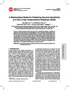
1. Introduction. Background information. Seawater has been injected into the naturally fractured Ekofisk chalk reservoir in the North Sea for nearly 20 years with great success. Many laboratory studies of spontaneous imbibition tests with chalk cores indicate that seawater has the potential to improve oil recovery. This has motivated for a number of experimental studies where the oil recovery for different core plugs is studied as a function of brine composition and temperature [37, 39, 38, 4, 5, 46, 40, 47]. 2+ seem to In particular, it has been observed that the ions Mg2+ , SO2− 4 , and Ca play an important role. By varying the concentration of these ions (one at a time) in seawater like brines, different oil recovery curves are produced. In order to illustrate this, we briefly review some highly interesting experimental spontaneous imbibition results reported in [46, 47]. In Fig. 1 oil recovery curves for some imbibition experiments with chalk core plugs are shown. In the left figure results for brines with varying concentrations of SO2− are shown. In particular, for a fixed temperature 4 of T = 130◦ C it is observed that increasing the amount of SO2− 4 ions gives a higher oil recovery level. Similar observations can be made from the right figure. One observation is that increasing the temperature for a given brine tends to increase the oil recovery. Another is that for a temperature at T = 100◦ C, adding Mg2+ ions to the imbibing brine leads to a strong increase in the oil recovery. When temperature is T = 130◦ C, this increase in oil recovery is amplified. This characteristic behavior also seems to depend on the amount of SO2− 4 ions that are present. In view of these experimental observations the purpose of this paper is to deal with the following questions: • Firstly, how to explain that different (steady state) oil recovery levels are reached depending on the chosen brine composition? What is the fundamental mechanism behind this behavior? • Secondly, how to explain that increase of respectively, SO2− ions and Mg2+ 4 ions in the imbibing brine, give higher oil recovery levels? Main idea. More precisely, the objective of this work is to bring forth a mathematical model that can allow for systematic and quantitative studies of the relation between brine composition and produced oil as observed in a lab scale setting. This will be achieved by combining two different modeling components: (i) Modeling of water-rock interaction in the context of geo-chemistry. (ii) Modeling of two-phase water-oil transport effects by means of relative permeability and capillary pressure curves. Highly sophisticated models have been developed for description of water-rock interaction governed by various transport effects (convective transport, molecular diffusion, mechanical dispersion, etc), see for example [25, 36, 29, 31] and references therein for a nice overview of this very active research field. However, this research is typically in the context of water-ion-mineral systems (single-phase systems). On the other hand, petroleum research has been a driving force behind development of modeling of two-phase water-oil transport (more generally, multiphase flow in porous media) [15]. Modeling and experimental activity have walked hand in hand for decades. See for instance [35, 18, 34] for some interesting and recent examples where modeling and experimental activity are both included in the study of spontaneous imbibition processes on lab scale. However, the coupling between (i) and (ii) seems to be more rare. It is our belief that we have to carefully design

PHYSICO-CHEMICAL MODELLING

70

70 SW−0S SW−1/2S SW SW−2S SW−4S

o

50

40

30

40

30

20

20

10

10

2

4

6

8

Time (days)

10

12

130 C

100 C Sw0x0S, add Mg at 53 days Sw0x2S, add Ca at 43 days Sw0, add Mg at 43 days Sw0x4S, add Mg at 53 days

50

0

o

o

70 C 60

Oil Recovery (%)

Oil Recovery (%)

60

0

3

14

0

0

20

40

60

80

100

120

Time (days)

Figure 1. Left: Oil recovery curves for imbibition tests on chalk concentrations in the cores performed at 130◦ C at various SO2− 4 imbibing fluids. SW represents seawater whereas SW-0S represents seawater without SO2− 4 , SW-2S represents seawater with 2 times seawater concentration of SO2− 4 , and so on. Right: Oil recovery curves for imbibition tests on chalk cores where Mg2+ or Ca2+ are added to the imbibing brine. Sw0 represents seawater without Mg2+ and Ca2+ whereas Sw0x0S is the same seawater but without 2− SO2− 4 , Sw0x2S contains 2 times seawater concentration of SO4 , and so on. Change of temperature is also involved. Figures have been reproduced, respectively, from the work [46] (left figure) and [47] (right figure) by the accuracy of an eye and must be considered as approximate. models that combine (i) and (ii) in an appropriate manner in order to obtain models that can explain the relation between oil recovery curves and brine composition, as reflected by Fig. 1. At this stage, as far as the core scale model is concerned, various simplifications will be done in order to not arrive at an overly complicated model with many different parameters that can be tuned. However, the hope is that yet the model will be sophisticated enough to suggest nontrivial mechanisms that possibly play a role in the relatively complicated physico-chemical system we are dealing with. In particular, a mathematical model that integrates (i) and (ii) can represent a helpful tool for improved understanding of the experimental results. The main idea we have implemented is formulation of a mathematical model that includes: • two phase water-oil displacement (pressure driven and/or capillary driven); • aqueous chemistry and water-rock interaction; • dynamic wettability alteration, in terms of changes in relative permeability and capillary pressure curves, that is linked to the water-rock interaction. In view of calculations based on thermodynamic equilibrium chemistry [21, 22] where a linear correlation between oil recovery and dissolution of calcite is obtained, a natural choice is to link wettability alteration to dissolution of calcite. This line will be pursued in this work. However, it should be noted that the framework we

4


work within is general enough to explore different possible relations between waterrock interaction (dissolution/precipitation and/or surface chemistry) and changes in the flow functions (relative permeability and capillary pressure). A key point in the present work is to link the water-rock chemistry to changes in the wetting state. In particular, we do no attempt to include details of the oil chemistry. Oil chemistry is implicitly taken care of in a more rough sense by the use of an interpolation function that gradually changes the saturation dependent flow functions according to changes in the mineral composition, see Remark 2 for further motivation. Previous works. In fact, the model developed in this work represents a proper combination of two models that previously have been proposed, respectively for the study of dynamic wettability alteration [44, 45] and chalk weakening effects due to water-rock interaction [16]. A 1D model for simulation of dynamic wettability alteration in spontaneous imbibition was developed in [44]. See also [43, 23] for similar type of models in the context of low salinity waterflooding on reservoir scale. The model in [44] represents a core plug on laboratory scale where a general wettability alteration (WA) agent is added. The term WA agent is used to represent a single ion or group of ions. In particular, we truncate all the complicated chemical interactions into a single adsorption function. Relative permeability and capillary pressure curves are constructed by employing an interpolation between two sets of generic curves corresponding to oil-wet (mixed wet) and water-wet conditions. Gradually, as the adsorption of the WA agent takes place, there is a shift towards more water-wetness resulting in a corresponding higher oil recovery. The form of the model is as follows (dimensionless form): st + f (s, c)x = ε([−λo f ](s, c)Pc (s, c)x )x (sc + a(c))t + (cf (s, c))x = δ(D(s)cx ) + ε(c[−λo f ](s, c)Pc (s, c)x )x ,

(1)

where s is water saturation, c concentration of WA agent, f is fractional flow function, λo is oil mobility, Pc capillary pressure, D(s) molecular diffusion coefficient, a(c) adsorption isotherm, whereas ε and δ are dimensionless characteristic numbers. Models of the form (1) have been studied extensively before in connection with for example polymer and surfactant flooding. A nice overview of this activity is given in the book [8] which also includes a comprehensive reference list. A special feature of the model is that the adsorption process, described by a standard adsorption isotherm (see [44]), makes the rock saturated by the WA agent after some time if there is a steady transport of this agent into the core. This in turn implies that the same wettability change will take place throughout the whole core independent of the specific ion concentrations of the brine that is used. It is only a question about how long time this wettability changing process will take. In other words, after an initial transient period, the oil recovery curves will reach the same steady state level. Consequently, such a model cannot be used to explain the experimental results shown in Fig. 1 where different brine compositions give different levels of oil recovery. This observation suggests that a more detailed description of relevant water-rock chemistry should be taken into account. On the other hand, in [16] a water-rock system was studied for the purpose of describing some recent experimental results where chalk cores were flooded with different brines. A main purpose was to investigate changes in ion concentrations measured at the outlet when cores were flooded with seawater like brines at a temperature T = 130◦ C. It was observed that the proposed model, which accounted


5

for combined flow and chemical reactions, could reproduce main trends of the measured ion concentrations at the outlet. A special feature of the model is that different brines give different long-time steady-state type of solutions. A main idea of the present work is to link wettability alteration to this brine-dependent steady-state behavior. Thus, in the current work we adopt this model for the oil-water-ion-mineral system in question. Compared to [16], we have to take into account the water-oil transport mechanisms in an appropriate manner as well as provide a link between the flow functions required for the water-oil transport (relative permeability and capillary pressure) and the water-rock interaction. For that purpose we rely on an approach similar to that used in [44, 43, 23] but where the role played by adsorption of the WA agent now is replaced by dissolution of calcite. This is done by introducing a wettability index H(ρc ) (lying between 0 and 1) that senses where the dissolution of calcite takes place. Results. The main contribution of the paper is: • Formulation of the model that incorporates the essential components required for systematic investigations of the combined effect of two-phase transport mechanisms and water-rock interaction. • Provide a first evaluation of the model. The 1D model we run is not directly comparable with the setting of most of the experimental results which involve flow in 2D or 3D geometries. However, we are interested in generic features like oil recovery curves as a function of brine composition and/or temperature. The numerical investigations demonstrate that different oil recovery levels are produced depending on the brine composition. More precisely, for a fixed set of parameters (flow and chemical reaction related parameters) the model predicts increasing oil recovery levels for higher concentration of SO2− 4 ions, similarly to the results reflected by Fig. 1 (left). Moreover, the strong enhanced oil recovery effect obtained by increasing the concentration of Mg2+ is also captured by the model, see Fig. 1 (right). The model also naturally reflects that temperature plays a crucial role for the resulting oil recovery curve. Consequently, we may conclude that the proposed model demonstrates that the relation between oil recovery curves and brine composition possibly can be understood as a result of the combined effect of transport (molecular diffusion), water-rock interaction in terms of dissolution/precipitation of minerals, and a corresponding wettability alteration due to dissolution of calcite. The structure of this paper is as follows: In Section 2 we first give a brief overview of the essential ingredients of the model. In Section 3 we describe the equations relevant for the aqueous equilibrium chemistry, as well as non-equilibrium waterrock chemistry (dissolution/precipitation). In Section 4 we describe the saturation dependent flow functions, relative permeability and capillary pressure, typically used for modeling of two-phase transport effects. In particular, we describe an interpolation mechanism that relates dissolution of calcite to a change of the wetting state represented by the relative permeability and capillary pressure functions. The full model where convective and diffusive transport effects are included, together with the water-rock interaction, is described in Section 5. In Section 6 we sketch the numerical approach employed for solving the resulting model (8) and (9), based on an operator splitting approach. Finally, in Section 7 we provide a first evaluation of the model by computing solutions for cases where we change the concentration, 2+ , and temperature for a seawater like brine. respectively, of SO2− 4 , Mg

6


2. The model. In this section we briefly define the oil-water-ion-mineral system we shall work with relevant for spontaneous imbibition lab experiments for chalk core plugs. The details of the derivation of the model are given in Section 3–5. We closely build upon the model that was developed in [16] for the study of a water-ionrock system. However, compared to that work we now have to consider an extended model where also the oil phase is included. For the modeling of two-phase water-oil transport we follow the approach described in [44], see also references therein. Let Ω be the domain of calcite CaCO3 and define the molar concentrations of the different species in the units of mol/liter: ρca = [Ca2+ ] ρmg = [Mg2+ ] ρso = [SO2− 4 ] ρna = [Na+ ] ρcl = [Cl− ]

ρc = [CaCO3 ] (solid) ρg = [CaSO4 ] (solid) ρm = [MgCO3 ] (solid) ρl = [H2 O] (water) ρo = [·] (oil)

(ions) (ions) (ions) (ions) (ions)

ρh = [H+ ] (ions) ρoh = [OH− ] (ions) ρhco = [HCO− 3 ] (ions) ρco = [CO2− ] (ions) 3

The domain Ω itself may depend on time, due to the undergoing chemical reactions which affect its surface. Currently, we neglect this dependence. Since we are including the bulk volume (matrix volume + pore volume) in the definition of the above densities, we will call them total concentrations. Later we shall define porous concentrations when dealing with porosity φ and volume fraction s for the water phase. The primary unknown concentrations are ρc , ρg , ρm , ρo , ρl , ρca , ρso , ρmg , ρna , ρcl , ρh , ρoh , ρco , and ρhco . We shall assume that the Na+ and Cl− ions do not take part in the chemical reactions, i.e., their concentrations ρna and ρcl are determined by the transport mechanisms only. We include chemical kinetics associated with the concentrations ρc , ρg , ρm , ρca , ρso , ρmg involved in the water-rock interactions (dissolution/precipitation), whereas the concentrations ρh , ρoh , ρco , and ρhco involved in the aqueous chemistry, are obtained by considering equilibrium state equations. In addition, a charge balance equation is included for the ions in question. Water-rock interaction (dissolution and precipitation). The model we shall study represents a reactive transport system with three mineral phases (CaCO3 , 2+ CaSO4 , MgCO3 ) and three aqueous species (Ca2+ , SO2− ) which react ac4 , Mg cording to basic kinetic laws. More precisely, the chemical reactions we include are: CaCO3 (s) + H+ Ca2+ + HCO− 3 2+

CaSO4 (s) Ca +

2+

MgCO3 (s) + H Mg

(dissolution/precipitation),

(2)

+

SO2− 4

(dissolution/precipitation),

(3)

+

HCO− 3

(dissolution/precipitation).

(4)

We shall take into account reaction kinetic relevant for these processes. Aqueous chemistry (chemical reactions in the water phase). Chemical reactions in the water phase are assumed to be at equilibrium. More precisely, in addition to (2)–(4), we will also make use of the following chemical reactions in or− + 2− der to determine concentrations of HCO− 3 , H , CO3 and OH (which are species


7

+ CO2 (g) + H2 O HCO− 3 +H ,

(5)

in the water phase): 2− + HCO− 3 CO3 + H , −

+

H2 O OH + H .

(6) (7)

We do not include reaction kinetic associated with these chemical reactions but assume that they are at equilibrium. In other words, it is implicitly assumed that they take place at a much faster time scale than the dissolution/precipitation processes (2)–(4). As mentioned, we shall also include a charge balance equation. Model for combined water-oil flow and water-rock interaction. The core plug under consideration is initially filled with formation water which is in equilibrium with the minerals inside the pore space. Moreover, initially, the wetting state is assumed to be such that no water will imbibe into the core when it is placed in water. However, when a brine with ion concentrations different from the formation water is used, there will be a transport of various ions into the core due to molecular diffusion. This creates concentration fronts that move with a certain speed. At these fronts, as well as behind them, chemical reactions will take place, both within the aqueous phase as well as on the rock surface. It is expected that the water-rock interaction then will lead to a change of the wetting state [37, 39, 38, 4, 5, 46, 40, 47]. The model that is formulated should be general enough to explore different hypothesis about possible links between water-rock interaction and changes in the wetting state. However, the main focus of this paper is to build into the model a mechanism that relates wettability alteration (towards a more water-wet state) to dissolution of calcite, see [22] for further motivation. We follow along the line of previous studies, see for example [1, 2, 3, 9, 10, 44] and references therein, and formulate a one-dimensional model. More precisely, the model we shall deal with takes the following form: (φs)t + γF (s, ρc )x = ε(AJ(s, ρc )x )x , (φsCna )t + γ(Cna F (s, ρc ))x = (DCna,x )x + ε(Cna AJ(s, ρc )x )x , (φsCcl )t + γ(Ccl F (s, ρc ))x = (DCcl,x )x + ε(Ccl AJ(s, ρc )x )x , (φsCca )t + γ(Cca F (s, ρc ))x = (DCca,x )x + ε(Cca AJ(s, ρc )x )x + τ (r˙c + r˙g ), (φsCso )t + γ(Cso F (s, ρc ))x = (DCso,x )x + ε(Cso AJ(s, ρc )x )x + τ r˙g ,

(8)

(φsCmg )t + γ(Cmg F (s, ρc ))x = (DCmg,x )x + ε(Cmg AJ(s, ρc )x )x + τ r˙m , (ρc )t = −τ r˙c , (ρg )t = −τ r˙g , (ρm )t = −τ r˙m . Here γ and ε are dimensionless positive constants, sometimes referred to as, respectively, the gravity number and capillary number. All the details leading to this model are given in thepsubsequent sections. In the model (8), a characteristic time τ and length scale L = Dm τ have been introduced. The unknown variables we solve for are water saturation s (dimensionless), and concentrations Cna , Ccl , Cca , Cso , Cmg , ρc , ρg , ρm (in terms of mole per liter water). Moreover, F (s, ρc ) is the fractional flow functions, D = D(φ, s) the molecular diffusion coefficient, A = A(s, ρc ) is the coefficient associated with capillary diffusion, and J(s, ρc ) is the so-called

8


Leverett function known from the Buckley Leverett theory. The dependence on the calcite concentration ρc involved in these functions is due to the proposed coupling between wettability alteration and dissolution of calcite. In addition, we must specify rate equations r˙k = r˙k (Cca , Cso , Cmg , Cna , Ccl ) for k = c, g, m. Following [9, 10, 16], and references therein, the reaction terms take the form h i r˙c = k1c sgn+ (ρc )Fc+ (Cca , Cso , Cmg ) − Fc− (Cca , Cso , Cmg ) , i h r˙g = k1g sgn+ (ρg )Fg+ (Cca , Cso , Cmg ) − Fg− (Cca , Cso , Cmg ) , (9) i h + − r˙m = k1m sgn+ (ρm )Fm (Cca , Cso , Cmg ) − Fm (Cca , Cso , Cmg ) , where the functions Fc , Fg , and Fm represent the kinetics of the precipitation and dissolution processes in question and k1c , k1g , and k1m are corresponding reaction rate constants. Here FI = FI+ − FI− , I = c, g, m, is a decomposition of F into its positive and negative parts, whereas sgn(x)+ = 1 if x > 0, otherwise it is 0. FI < 0 represents precipitation, whereas FI > 0 represents dissolution. The above formulation takes into account that a mineral can be dissolved only as long as it exists, and is similar to what has been done in other works, see for example [9, 33] and references therein. Ck represents porous concentrations and are related to the total concentrations by ρk = φsCk , for k = ca, so, mg, na, cl.

3. The model for water-rock interaction. In the following, we first give some more details concerning the equilibrium chemistry associated with the chemical reactions (5)–(7), the aqueous chemistry. Then we describe the relations that take into account kinetics associated with the precipitation/dissolution processes (2)–(4). In particular, we shall distinguish between concentration C and chemical activity a noting that they are related by a = γC,

(10)

where γ is the activity coefficient. According to the Debuye-H¨ uckel equation, see for example [25, 32], the activity coefficient γi is given by √ AZi2 I0 √ , − log10 (γi ) = (11) 1 + a0i B I0 where the index i refers to the different species involved in the system which is studied. Moreover, Zi refers to the ionic charges, A(T ) and B(T ) are temperature dependent given functions [20, 21], similarly for the constants a0i , whereas I0 refers to the ionic strength defined by I0 =

1X Ci Zi2 . 2 i

(12)

For the numerical calculations, we calculate I0 based on the ion concentrations for the imbibing brine. Consequently, I0 is assumed to be constant throughout the imbibition process. Since the temperature is kept constant, the activity coefficients are also taken to be constant, according to (11).


9

3.1. Aqueous chemistry. In the subsequent discussion we assume that we know the concentrations Cna and Ccl . Based on this we shall discuss the various equations associated with the chemical reactions described by (5)–(7). We assume that the CO2 partial pressure PCO2 is known, from which the CO2 concentration can be determined. More precisely, the local equilibrium associated with (5) gives the relation C1 = PCO2 K = ahco ah = (γhco γh )Chco Ch ,

(13)

for an appropriate choice of the equilibrium constant (solubility product) K and partial pressure PCO2 . The chemical reaction equation (6) gives us ³γ γ Ć C aco ah co h co h C2 = = , (14) ahco γhco Chco where C2 is a known solubility constant. Moreover, the reaction equation (7) gives Cw = ah aoh = (γoh γh )Coh Ch ,

(15)

where Cw is known. The following aqueous charge balance equation is also assumed to hold for the various species contained in the water phase X Ci Zi = 0, (16) i

where Zi refers to the ionic charge of species i. For the system in question, this results in the following balance equation: 2Cca + 2Cmg + Ch + Cna = 2Cso + Chco + 2Cco + Coh + Ccl .

(17)

Thus, the four equations (13)–(16) allow us to solve for Ch , Chco , Cco , and Coh . This relation can be written in the form C3 = Chco + 2Cco + Coh − Ch ,

(18)

where C3 = C3 (Cca , Cmg , Cso ; Cna , Ccl ) = 2(Cca + Cmg − Cso ) + (Cna − Ccl ).

(19)

It’s convenient to introduce the following notation: e1 = C1 , e2 = C2 γhco , ew = Cw . C C C (20) γhco γh γco γh γh γoh We shall make use of the simplifying assumption that the concentration Cco of CO2− is relatively low and can be neglected in the charge balance equation (18). 3 Clearly, (18) can then be written in the form ew C C3 = Chco + − Ch , (21) Ch where we have used (15). Combining (13) and (21) we get e1 + C ew C C3 = − Ch , Ch e1 + C ew ) = 0. The relevant which results in the second order equation Ch2 +C3 Ch −(C solution is then given by q ´ e1 1³ C e1 + C ew ) , −C3 + C32 + 4(C . Ch = (22) Chco = 2 Ch Finally, Cco and Coh can be determined from the equations (14) and (15). In particular, we note that Ch = Ch (Cca , Cso , Cmg ; Cna , Ccl ), in view of (19).

10


3.2. Rate equations for the water-rock interaction. The rate equations associated with the water-rock interaction, as described by the dissolution/precipitation processes (2)–(4), are obtained by following an approach similar to that in [9, 16], see also references therein like [25] (chapter 1) and [36, 29]. The main point of this approach is the use of an empirical rate equation of the form R = k(1 − Ω)n ,

(23)

where R is the rate, k and n are empirical fitting terms and (1 − Ω) the degree of disequilibrium with the mineral in question. Ω is the ratio of the ion activity product (IAP) to the solubility product K for the solid in question, that is, Ω = IAP/K. If 0 < 1 − Ω the solution is undersaturated which may lead to dissolution; if 0 > 1 − Ω the solution is supersaturated which implies precipitation. Thus, the reaction terms r˙i , for i = c, g, m associated with (2)–(4), are given as follows where we have used n = 1 in (23): ³ ³ ahco aca ´ γca γhco Cca Chco ´ c aca ahco c = k1c 1 − r˙c = k1c ac − k−1 = k 1 − 1 ah K c ah γ h Ch K c (24) ³ ´ γca C1 Cca = k1c 1 − 2 c 2 , γh K Ch ³ aca aso ´ g g r˙g = k1 ag − k−1 aca aso = k1g 1 − Kg (25) ³ γca γso Cca Cso ´ g , = k1 1 − Kg ³ ³ a ahco amg ´ γmg γhco Cmg Chco ´ m mg ahco m r˙m = k1m am − k−1 = k1m 1 − = k 1 − 1 ah K m ah γ h Ch K m ³ ´ γmg C1 Cmg = k1m 1 − 2 m 2 , γ h K Ch (26) where Kc =

k1c c , k−1

Kg =

k1g g , k−1

Km =

k1m m . k−1

(27)

Here aj represents chemical activity associated with species j. Moreover, we have supposed that the minerals exist as pure phases which implies that the ion activities of the minerals are one, see for example [9]. That is, we have set ac = ag = am = 1 in (24)–(26). Mixed phases can be accounted for but that is an unnecessary comj plication at the present stage. k−1 represents the rate of precipitation whereas k1j represents the rate of dissolution associated with the different species j = c, g, m corresponding to CaCO3 , CaSO4 , and MgCO3 . Similarly, K j is used to represent the equilibrium constant (solubility product) associated with j = c, g, m. These are known values. On the other hand, much less is known about the rate of precipitaj tion/dissolution represented by k1j and k−1 . It is convenient to introduce the notation ³ γca γhco Cca Chco ´ def , Fc (Cca , Cso , Cmg ; Cna , Ccl ) := 1 − γh Ch K c ³ γca γso Cca Cso ´ def (28) Fg (Cca , Cso ; Cna , Ccl ) := 1 − , Kg ³ ´ γmg γhco Cmg Chco def Fm (Cca , Cso , Cmg ; Cna , Ccl ) := 1 − . γh Ch K m


11

Then we get the following rate equations associated with the minerals represented by ρc , ρg , and ρm : dρc = −r˙c = −k1c Fc (Cca , Cso , Cmg ; Cna , Ccl ), dt dρg = −r˙g = −k1g Fg (Cca , Cso , Cmg ; Cna , Ccl ), dt dρm = −r˙m = −k1m Fm (Cca , Cso , Cmg ; Cna , Ccl ). dt

(29)

Similarly, (24)–(26) give rise to the following set of rate equations associated with the aqueous species ρca , ρso , and ρmg involved in the precipitation/dissolution processes (2)–(4): dρca = r˙ca = r˙c + r˙g = k1c Fc (Cca , Cso , Cmg ; Cna , Ccl ) + k1g Fg (Cca , Cso , Cmg ; Cna , Ccl ), dt dρso = r˙so = r˙g = k1g Fg (Cca , Cso , Cmg ; Cna , Ccl ), dt dρmg = r˙mg = r˙m = k1m Fm (Cca , Cso , Cmg ; Cna , Ccl ). dt (30) An important modification is to take into account the fact that mineral dissolution stops once the mineral has disappeared [9, 16]. To build this mechanism into the rate equations given by (24)–(26), we use (28) and change these equations in the following manner: h i r˙c = k1c sgn+ (ρc )Fc+ (Cca , Cso , Cmg ) − Fc− (Cca , Cso , Cmg ) , i h r˙g = k1g sgn+ (ρg )Fg+ (Cca , Cso , Cmg ) − Fg− (Cca , Cso , Cmg ) , (31) h i + − r˙m = k1m sgn+ (ρm )Fm (Cca , Cso , Cmg ) − Fm (Cca , Cso , Cmg ) , where

½ +

sgn (x) = FI = FI+ − FI− ,

1, 0,

if x ≥ 0; otherwise,

where FI+ = max(0, FI ),

FI− = max(0, −FI ).

Clearly, in view of (29), we see that for FI < 0 where I = c, g, m represents the mineral in question, the mineral precipitates; for FI = 0 chemical equilibrium exists and nothing happens; for FI > 0 the mineral dissolves, but only as long as the mineral exists, i.e., ρI > 0. 4. Coupling of wettability alteration to changes on the rock surface. This section discusses aspects concerning the flow functions (relative permeability and capillary pressure) and partially follows ideas employed in previous works [44, 43, 23]. 4.1. Relative permeability and capillary pressure functions. As a basic model for relative permeability functions the well-known Corey type correlations

12


are used [15]. They are given in the form (dimensionless functions) ³ s−s Ń k wr k(s) = k ∗ , swr ≤ s ≤ 1 − sor , 1 − sor − swr (32) ³ 1 − s − s Ń k o or ko (s) = ko∗ , swr ≤ s ≤ 1 − sor , 1 − sor − swr where swr and sor represent critical saturation values and N k and N ko are the Corey exponents that must be specified. In addition, k ∗ and ko∗ are the end point relative permeability values that also must be given. As a simple model for capillary pressure a piecewise linear function of the following form is used:  1 ³ s < swr ,   ´   pc1 −1  swr ≤ s ≤ s1 ,  1 + s³1 −swr (s´− swr )  pc2 −pc1 ∗ Pc (s) = C s1 ≤ s ≤ s2 , (33) pc1 + s2 −s1 (s − s1 )  ³ ´   −1−pc2  pc2 + 1−s (s − s2 ) s2 ≤ s ≤ 1 − sor ,   or −s2   −1 s > 1 − sor , where C ∗ and the points (s1 , pc1 ) and (s2 , pc2 ) are constants that must be specified. In a more realistic setting these would be based on experimental data and, typically, more than two points would be given. Furthermore, C ∗ is a scaling constant (characteristic capillary pressure) that contains information about interfacial tension and contact angle effects. More precisely, Pc (s) = C ∗ J(s), where the dimensionless function J(s) is called the Leverett function and its multiplier C ∗ takes the form [8, 35, 18] σ cos(θ) , (34) C∗ = p κ/φ where σ is interfacial tension, θ is contact angle, κ absolute permeability, φ porosity. In the following data required to obtain concrete relative permeability and capillary pressure curves are specified that can represent, respectively, oil-wet and water-wet conditions. Note that more precisely, spontaneous imbibition experiments have been carried out for preferential oil-wet chalk cores [46, 47] (also referred to as mixed wet conditions) but for simplicity we employ the word ”oil-wet”. Oil-wet conditions. The following set of values for oil-wet conditions is used: ow ow k ∗,ow = 0.7, ko∗,ow = 0.75, sow = 2, wr = 0.1, sor = 0.15, N k

N koow = 3. (35)

Applying these values in (32) the following two relative permeability curves are obtained ow k ow (s; sow wr , sor ),

ow koow (s; sow wr , sor ),

ow for sow wr ≤ s ≤ 1 − sor .

Similarly, from (33) a corresponding capillary pressure function is obtained ow Pcow (s; sow wr , sor ),

ow for sow wr ≤ s ≤ 1 − sor ,

where the following values are used ow (sow 1 , pc1 ) = (0.2, −0.1), ∗

ow (sow 2 , pc2 ) = (0.8, −0.5).

(36)

Moreover, C is associated with a reference capillary pressure value which we denote by Pc,r C ∗,ow = Pc,r . (37)


Pc series

Kr series 1

1

oil−wet water−wet

0.8

0.6

0.7

0.4

0.6 0.5 0.4 0.3

0.2 0 −0.2 −0.4

0.2

−0.6

0.1

−0.8 0

0.2

0.4

0.6

0.8

oil−wet water−wet

0.8

Capillary Pressure

Relative Permeability

0.9

0

13

1

−1

0

0.2

Sw

0.4

0.6

0.8

1

Sw

Figure 2. Left: Example of relative permeability curves corresponding to oil-wet and water-wet conditions. Right: Example of capillary pressure curves corresponding to oil-wet and water-wet like conditions. A specific value for Pc,r is given in Section 7. We refer to Fig. 2 for a plot of these curves (red line). For the numerical calculations in Section 7 we shall choose initial water saturation sinit such that Pcow (sinit ) ≈ 0, i.e. sinit = 0.19. This implies that no spontaneous imbibition will take place when we start with a core plug that initially is described by Pcow given by (33) and (36) corresponding to an oil-wet state. Water-wet conditions. The following set of values for water-wet conditions is used: ww ww k ∗,ww = 0.4, ko∗,ww =0.9, sww = 3, N koww = 2. (38) wr = 0.15, sor = 0.25, N k

These choices give corresponding relative permeability curves ww k ww (s; sww wr , sor ),

ww koww (s; sww wr , sor ),

ww for sww wr ≤ s ≤ 1 − sor ,

and via (33) a corresponding capillary pressure function ww Pcww (s; sww wr , sor ),

ww for sww wr ≤ s ≤ 1 − sor ,

with ww (sww 1 , pc1 ) = (0.2, 0.4),

ww (sww 2 , pc2 ) = (0.7, 0).

(39)

Again C ∗,ww = Pc,r . We refer to Fig. 2 for a plot of these curves (blue line).

(40)

Remark 1. Starting with an initial oil-wet core plug represented by flow functions Pc = Pcow , k = k ow , and ko = koow and an initial saturation sinit such that Pcow (sinit ) = 0, it’s clear that no more oil will come out of the core plug. However, due to molecular diffusion, and the fact that the initial brine in the core plug (formation water) is different from the brine in which the plug is placed, the different ions will move into the core. This creates a non-equilibrium state in the core where the ion concentrations are not in equilibrium with the rock. In particular, this generates chemical reactions in terms of dissolution/precipitation that change the rock surface. In this work we propose to link alteration of the wetting state to these changes in the rock surface.

14

S. EVJE AND A. HIORTH Weighting function H(m) 1 H(m)

0.9 0.8 0.7

H(m)

0.6 0.5 0.4 0.3 0.2 0.1 0

0

0.01

0.02

0.03

0.04

0.05

m

Figure 3. The weighting function H(m) as defined by (41) with r = 400. The choice of r determines how much calcite that must be dissolved to bring forth a certain change of the wetting state. Note that the function H(m) quickly falls off from 1. This means that the initial dissolution will create a larger wettability alteration. Further dissolution will have less impact on the change of the wetting state. Different possible links between changes in the mineral composition and alteration of the wetting state is of course possible. The objective of this paper is to explore the hypothesis that dissolution of calcite is a governing force in this process, based on some previous calculations [21, 22]. The implementation of this mechanism in the model is the topic of the subsequent subsection. 4.2. Dissolution of calcite as a mechanism for wettability alteration. Having an initial concentration ρ0 of a mineral with concentration ρ, we define the quantity m(ρ) m(ρ) := max(ρ0 − ρ, 0) as a measure for the dissolved mineral. Moreover, we define H(ρ) :=

1 , 1 + rm(ρ)

(41)

where r > 0 is a specified constant. In the numerical investigations we use r = 400. The function H(ρ) then becomes a weighting function such that (i) 0 < H(ρ) ≤ 1,

for ρ ≥ 0;

(ii) H(ρ) = 1,

for ρ ≥ ρ0 (no dissolution or precipitation);

(iii)

0 < H(ρ) < 1

for ρ < ρ0 (dissolution).

How fast H(ρ) is approaching 0 as m(ρ) is increasing, depends on the choice of r. Now, the weighting function H(ρ) can be used to represent the wetting state in the core plug; H(ρ) = 1 corresponds to the initial oil-wet state, whereas H(ρ) ≈ 0 represents the water-wet state. By defining relative permeability and capillary pressure curves by means of the weighting function H(ρ) as described in the next subsection, the model can account for a dynamic change from an initial oil-wet state towards a water-wet state controlled by the degree of dissolution of calcite that takes place inside the core.


15

Remark 2. The interpolation function H(ρ) defined by (41) represents the average wetting state of the porous media inside a representative elementary volume (REV) [7]. The mathematical form can be motivated by making the following two assumptions: 1. There is a constant number of calcium sites at the pore surface, which is denoted ΓT Ca . 2. The wettability change reaction at the surface is described by the following chemical reaction: >CaR-COO0 + X+ + H2 O >CaH2 O+ ,

(42) −

where > means that the reaction takes place at the surface. R-COO is an organic ion, and >CaR-COO0 is a surface complex consisting of calcium cites at the surface and >CaH2 O+ and R-COO− ions from the oil phase. Hence, the concentration of >CaR-COO0 characterizes the wetting state. In particular, a decrease in the concentration of >CaR-COO0 (i.e. higher concentration of >CaH2 O+ ) indicates a wettability change towards a more water wet surface. X is a chemical species that facilitates release of organic compounds attached to the surface. From Assumption 1 above we can write the following equation: ΓT Ca = Γ>CaH2 O+ + Γ>CaR-COO0 ,

(43)

i.e. the total number of calcium sites is the sum of the concentration of free calcium cites (Γ>CaH2 O+ ) and the calcium sites with adsorbed organic ions (Γ>CaR-COO0 ). Assumption 2 gives the following equilibrium equation: K =

Γ>CaH2 O+ . Γ>CaR-COO0 mX

(44)

Here the activity of H2 O is equal to one and mX is the concentration of X. By combining equation (43) and (44), we get: Γ>CaR-COO0 =

ΓT Ca . 1 + mX K

(45)

Comparing this equation with equation (41), we find that H(ρ) = Γ>CaR-COO0 /ΓT Ca when mX is associated with m = max(ρ0 − ρ, 0), and K = r. In other words, H coincides with Γ>CaR-COO0 when it is normalized relatively the total number of calcium sites ΓT Ca . The function H(ρ) falls quite rapidly off from 1 when m increases, see Fig. 3. This indicates that the dissolution will preferentially take place where the oil is adsorbed to the rock surface. In [42] p.162, it is stated that a reaction of the type (42) tends to enhance the dissolution, which could support the proposed functional behavior. 4.3. Modeling of transition from oil-wet to water-wet conditions. Improved oil recovery by invasion of seawater in a preferential oil-wet porous medium is ultimately due to changes in various flow parameters. The flow conditions before and after the wettability alteration can be described by capillary pressure curves, relative permeability curves, and residual saturations. In this work wettability alteration is incorporated in these flow parameters by defining capillary pressure Pc (s, ρc ) and relative permeability curves k(s, ρc ), ko (s, ρc ) through an interpolation between the oil-wet and water-wet curves given in (32)–(40).

16


More precisely, motivated by the proposed hypothesis that transition from preferential oil-wet towards water-wet conditions depends on the dissolution of CaCO3 , the following interpolation is proposed: k(s, ρc ) = H(ρc )k ow (s) + [1 − H(ρc )]k ww (s),

(46)

where H(ρc ) is defined by (41) and ρc is the calcite concentration. Hence, when no dissolution of CaCO3 has taken place it follows that H(ρc ) = 1, implying that k(s, ρc ) = k ow (s). This reflects the initial preferential oil-wet wetting state. Then, as dissolution of CaCO3 takes place, it follows that m(ρc ) increases. In particular, if the dissolution effect m(ρc ) becomes large enough H(ρc ) ≈ 0, which means that k(s, ρc ) ≈ k ww (s), reflecting that a wettability alteration has taken place which results in a water-wet wetting state. The same interpolation procedure is natural to use for the capillary pressure curve. That is, Pc (s, ρc ) = H(ρc )Pcow (s) + [1 − H(ρc )]Pcww (s).

(47)

Thus, different concentrations of ρc below its initial concentration ρc,0 as measured by m(ρc ), produce capillary pressure curves that lie between the two extremes Pcow and Pcww . 5. The coupled water-oil flow and chemical reaction model. In a more complete description we also want to take into account convective and diffusive forces associated with the brine as well as the oil phase. In order to include such effects we must consider the following equations for the total concentrations ρo , ρl , ρca , ρso , ρmg , ρna , ρcl , ρc , ρg , ρm : ∂t ρo + ∇ · (ρo vo ) = 0,

(oil flowing through the pore space)

∂t ρl + ∇ · (ρl vl ) = 0,

(water flowing through the pore space)

∂t ρna + ∇ · (ρna vg ) = 0,

(Na+ -ions in water)

∂t ρcl + ∇ · (ρcl vg ) = 0,

(Cl− -ions in water)

∂t ρca + ∇ · (ρca vg ) = r˙c + r˙g ,

(Ca2+ -ions in water)

∂t ρso + ∇ · (ρso vg ) = r˙g ,

(SO2− 4 -ions in water)

∂t ρmg + ∇ · (ρmg vg ) = r˙m ,

(Mg2+ -ions in water)

∂t ρc = −r˙c ,

(precipitation/dissolution of CaCO3 )

∂t ρg = −r˙g ,

(precipitation/dissolution of CaSO4 )

∂t ρm = −r˙m ,

(precipitation/dissolution of MgCO3 ).

(48)

The first seven equations represent concentrations associated with the pore space, the last three equations are associated with the matrix. Here vo , vl and vg are, respectively, the oil, water and species ”fluid” velocities. The subsequent derivation of the model closely follows the work [16], however, we now have to account also for the oil phase. Let so denote the oil saturation, i.e. the fraction of volume of the pore space φ that is occupied by the oil phase, and s the corresponding water saturation. The two saturations are related by the basic relation so + s = 1. Furthermore, we define the porous concentration Co associated with the oil component as the concentration taken with respect to the volume of the pore space occupied by oil and represented by φso . Hence, Co and ρo are related by ρo = φso Co .

(49)


17

Similarly, the porous concentrations of the various components in the water phase are defined as the concentration taken with respect to the volume of the pores occupied by water φs. Consequently, the porous concentrations Cl , Cna , Ccl , Cca , Cmg , and Cso are related to the total concentrations by ρl = φsCl , ρna = φsCna , ρcl = φsCcl , ρca = φsCca , ρmg = φsCmg , ρso = φsCso . Following Aregba-Driollet et al [1, 2, 3], we argue that since oil, water, and the ions in water Na+ , Cl− , Ca2+ , Mg2+ , and SO2− 4 flow only through the pores of the calcite specimen, the ”interstitial” velocity vo associated with the oil, vl associated with the water, and vg associated with the ions, have to be defined with respect to the concentrations inside the pores, and differ from the respective seepage velocities Vo , Vl and Vg . The velocities are related by the Dupuit-Forchheimer relations, see [2] and references therein, Vo = φso vo ,

Vl = φsvl ,

Vg = φsvg .

(50)

Consequently, the balance equations (48) can be written in the form ∂t (φso Co ) + ∇ · (Co Vo ) = 0, ∂t (φsCl ) + ∇ · (Cl Vl ) = 0, ∂t (φsCna ) + ∇ · (Cna Vg ) = 0, ∂t (φsCcl ) + ∇ · (Ccl Vg ) = 0, ∂t (φsCca ) + ∇ · (Cca Vg ) = r˙c + r˙g , ∂t (φsCso ) + ∇ · (Cso Vg ) = r˙g ,

(51)

∂t (φsCmg ) + ∇ · (Cmg Vg ) = r˙m , ∂t ρc = −r˙c , ∂t ρg = −r˙g , ∂t ρm = −r˙m . In order to close the system we must determine the seepage velocities Vo , Vl and Vg . For that purpose we consider the concentration of the water phase (brine) C that occupies the pore space as a mixture of water Cl and the various species Na+ , Cl− , Ca2+ , Mg2+ , and SO2− 4 represented by Cg . In other words, Cg = Cna + Ccl + Cca + Cmg + Cso ,

C = Cg + Cl .

(52)

Then, we define the seepage velocity V associated with C by CV := Cg Vg + Cl Vl .

(53)

Now we are in a position to rewrite the model in terms of V and the diffusive velocity Ug given by Ug = Vg − V.

(54)

18


Then the model (51) takes the form ∂t (φso Co ) + ∇ · (Co Vo ) = 0, ∂t (φsCl ) + ∇ · (Cl Vl ) = 0, ∂t (φsCna ) + ∇ · (Cna Ug ) = −∇ · (Cna V), ∂t (φsCcl ) + ∇ · (Ccl Ug ) = −∇ · (Ccl V), ∂t (φsCca ) + ∇ · (Cca Ug ) = (r˙c + r˙g ) − ∇ · (Cca V), ∂t (φsCso ) + ∇ · (Cso Ug ) = r˙g − ∇ · (Cso V),

(55)

∂t (φsCmg ) + ∇ · (Cmg Ug ) = r˙m − ∇ · (Cmg V), ∂t ρc = −r˙c , ∂t ρg = −r˙g , ∂t ρm = −r˙m . Furthermore, we can assume that the seepage velocity V associated with the water phase represented by C, is given by Darcy’s law [2, 6, 30] V = −κλ(∇p − ρg∇d),

λ=

k µ

(56)

where κ is permeability and µ is viscosity, and p pressure in water phase. Similarly, for the oil phase Vo = −κλo (∇po − ρo g∇d),

λo =

ko µo

(57)

The diffusive velocity Ug is expressed by Fick’s law by Cα Ug = −D∇Cα ,

α = na, cl, ca, so, mg,

D = (φp sq Dm + α|V|)I,

(58)

where Dm is the effective molecular diffusion coefficient, α is the dispersion length (longitudinal and transversal dispersion lengths are here taken to be equal), and I is the identity tensor. In view of (52) and (58), it follows that Cg Ug = −D∇Cg .

(59)

Note that we assume that the diffusion coefficient D is the same for all species α = na, cl, ca, so, mg. This is a reasonable assumption as long as the concentration is not too high, see e.g. [9]. Moreover, we shall apply the following simplified molecular diffusion coefficient (based on Archie’s law) D = Dm φp sq I,

1 ≤ p, q ≤ 2.5,

(60)

where the mechanical dispersion term is neglected since we focus on spontaneous imbibition. The coefficient p is referred to as the cementation exponent, q as the saturation exponent. The cementation exponent is often close to 2 whereas the saturation exponent is also often fixed at a value in the same range, see for example [11, 14, 7]. For the simulations we have used p = q = 1.9. Using (58) and (60) in


19

(55) yields ∂t (φso Co ) + ∇ · (Co Vo ) = 0, ∂t (φsCl ) + ∇ · (Cl Vl ) = 0, ∂t (φsCna ) − ∇ · (D∇Cna ) = −∇ · (Cna V), ∂t (φsCcl ) − ∇ · (D∇Ccl ) = −∇ · (Ccl V), ∂t (φsCca ) − ∇ · (D∇Cca ) = (r˙c + r˙g ) − ∇ · (Cca V), ∂t (φsCso ) − ∇ · (D∇Cso ) = r˙g − ∇ · (Cso V),

(61)

∂t (φsCmg ) − ∇ · (D∇Cmg ) = r˙m − ∇ · (Cmg V), ∂t ρc = −r˙c , ∂t ρg = −r˙g , ∂t ρm = −r˙m . In particular, summing the equations corresponding to Cna , Ccl , Cca , Cso , and Cmg , we obtain an equation for Cg in the form ∂t (φsCg ) − ∇ · (D∇Cg ) = (r˙c + 2r˙g + r˙m ) − ∇ · (Cg V).

(62)

In a similar manner, using Cl Vl = Cl V − Cg Ug (obtained from (53), (54), and (52)) in the second equation of (61), the following equation is obtained ∂t (φsCl ) + ∇ · (Cl V) = ∇ · (Cg Ug ).

(63)

Summing (63) and (62), we get the following equation for the concentration of the water phase with its different chemical components, represented by C = Cg + Cl , ∂t (φsC) + ∇ · (CV) = (r˙c + 2r˙g + r˙m ).

(64)

To sum up, we have a model in the form ∂t (φso Co ) + ∇ · (Co Vo ) = 0, ∂t (φsC) + ∇ · (CV) = (r˙c + 2r˙g + r˙m ), ∂t (φsCna ) + ∇ · (Cna V) = ∇ · (D∇Cna ), ∂t (φsCcl ) + ∇ · (Ccl V) = ∇ · (D∇Ccl ), ∂t (φsCca ) + ∇ · (Cca V) = ∇ · (D∇Cca ) + (r˙c + r˙g ), ∂t (φsCso ) + ∇ · (Cso V) = ∇ · (D∇Cso ) + r˙g ,

(65)

∂t (φsCmg ) + ∇ · (Cmg V) = ∇ · (D∇Cmg ) + r˙m , ∂t ρc = −r˙c , ∂t ρg = −r˙g , ∂t ρm = −r˙m , where D = D(φ, s) as given by (60). Simplifying assumptions. Before we proceed some simplifying assumptions are made: • The oil and water component densities Co and C are assumed to be constant, i.e., incompressible fluids; • The effect from the chemical reactions in the water phase equation (second equation of (65)) is neglected which is reasonable since the concentration of the water phase C is much larger than the concentrations of the ion exchange

20


involved in the chemical reactions, this is consistent with [16]. See [2, 3] for an air-rock system where this effect is not neglected; • Constant porosity φ, absolute permeability κ, viscosities µ, µo ; • One dimensional flow in a vertical domain. This results in the following simplified model where h is used to represent the spatial coordinate: ∂t (φso ) + ∂h (Vo ) = 0, ∂t (φs) + ∂h (V ) = 0, ∂t (φsCna ) + ∂h (Cna V ) = ∂h (D(φ, s)∂h Cna ), ∂t (φsCcl ) + ∂h (Ccl V ) = ∂h (D(φ, s)∂h Ccl ), ∂t (φsCca ) + ∂h (Cca V ) = ∂h (D(φ, s)∂h Cca ) + (r˙c + r˙g ), ∂t (φsCso ) + ∂h (Cso V ) = ∂h (D(φ, s)∂h Cso ) + r˙g ,

(66)

∂t (φsCmg ) + ∂h (Cmg V ) = ∂h (D(φ, s)∂h Cmg ) + r˙m , ∂t ρc = −r˙c , ∂t ρg = −r˙g , ∂t ρm = −r˙m , In view of (56) and (57) in a vertical 1D domain, we get V = − κλ[(p)h − ρg], Vo = − κλo [(po )h − ρo g],

k(s, ρc ) µ ko (s, ρc ) λo (s, ρc ) = , µo

λ(s, ρc ) =

(67) (68)

Here g is the gravity constant g = 9.81. Moreover, capillary pressure Pc (s, ρc ) is defined as the difference between oil and water pressure Pc (s, ρc ) = po − p, where Pc is a known function. Total velocity vT is given by ³ ´ vT := V + Vo = −κ λ[ph − ρg] + λo [(po )h − ρo g] ³ ´ = −κ λ[(po )h − (Pc )h − ρg] + λo [(po )h − ρo g] ³ ´ = −κ λT (po )h − λ(Pc )h − g[λρ + λo ρo ]

(69)

(70)

= −κλT (po )h + κλ(Pc )h + κg[λρ + λo ρo ], where total mobility λT λT = λ + λo ,

(71)

has been introduced. Summing the two first equations of (66) and using that 1 = s + so , implies that (vT )h = 0, i.e., vT =constant and is determined, for example, from the boundary conditions. From (70) it follows that Z h vT ´ 1 ³ λ(Pc )h + g[λρ + λo ρo ] − dh, (72) po = λT κ which can be used to obtain po once s and ρc are known. From the continuity equation for s given by the second equation of (66) it follows (since V = −κλ[(po )h −


(Pc )h − ρg])

21

³ ´ ³ ´ ³ ´ (φs)t + −κλ(po )h + κλ(Pc )h + κλρg = 0, h

h

(73)

h

where, in view of (70), −κ(po )h =

vT λ λ λo − κ (Pc )h − κg[ ρ + ρo ]. λT λT λT λT

Thus, ³ hv i´ λ λ λo T (φs)t + λ − κ (Pc )h −κg[ ρ + ρo ] λT λT λ λT h ³T ´ ³ ´ + κλ(Pc )h + κλρg = 0. h

(74)

h

The fractional flow function f (s, ρc ) and fo (s, ρc ) are defined as follows λ(s, ρc ) , λ(s, ρc ) + λo (s, ρc ) λo (s, ρc ) def fo (s, ρc ) := = 1 − f (s, ρc ). λ(s, ρc ) + λo (s, ρc ) def

f (s, ρc ) :=

(75) (76)

Using this in (74) implies that ´ ³ ´ ³ (φs)t + vT f (s, ρc )+κg∆ρ[f λ0 ](s, ρc ) − κ[λf ](s, ρc )(Pc )h −κλ(s, ρc )(Pc )h = 0, h

h

(77) where ∆ρ = [ρ − ρo ]. Noting from (75) that λf − λ = −λo f, (77) can be written in the form ³ ´ ³ ´ (φs)t + vT f (s, ρc ) + ∆ρκg[f λ0 ](s, ρc ) = − κ[λo f ](s, ρc )(Pc (s, ρc ))h . (78) h

h

The same procedure can be applied for the continuity equation for the different ions in water in (66). This gives the following equation for i = na, cl, ca, so, mg: ³ h i´ (φsCi )t + Ci vT f (s, ρc ) + ∆ρκg[f λ0 ](s, ρc ) h ³ ´ (79) = (D(s)Ci,h )h − κCi [λo f ](s, ρc )(Pc (s, ρc ))h + Reactioni , h

Thus, in view of (78) and (79), a model has been obtained of the form ∂t (φs) + ∂h F (s, ρc ) = ∂h (A(s, ρc )∂h Pc (s, ρc )),

(80)

∂t (φsCna ) + ∂h (Cna F (s, ρc )) = ∂h (D∂h Cna ) + ∂h (Cna A(s, ρc )∂h Pc (s, ρc )), ∂t (φsCcl ) + ∂h (Ccl F (s, ρc )) = ∂h (D∂h Ccl ) + ∂h (Ccl A(s, ρc )∂h Pc (s, ρc )), ∂t (φsCca ) + ∂h (Cca F (s, ρc )) = ∂h (D∂h Cca ) + ∂h (Cca A(s, ρc )∂h Pc (s, ρc )) + (r˙c + r˙g ), ∂t (φsCso ) + ∂h (Cso F (s, ρc )) = ∂h (D∂h Cso ) + ∂h (Cso A(s, ρc )∂h Pc (s, ρc )) + r˙g , ∂t (φsCmg ) + ∂h (Cmg F (s, ρc )) = ∂h (D∂h Cmg ) + ∂h (Cmg A(s, ρc )∂h Pc (s, ρc )) + r˙m , ∂t ρc = −r˙c , ∂t ρg = −r˙g , ∂t ρm = −r˙m , where

F (s, ρc ) = vT f (s, ρc ) + g∆ρκG(s, ρc ), A(s, ρc ) = −κG(s, ρc ).

G(s, ρc ) = [f λo ](s, ρc )

(81)

22


Counter-current flow. In the following we shall assume that the two-phase flow takes place as counter-current flow, i.e., the total velocity vT is zero inside the core, vT = 0. This assumption is reasonable in light of the fact that the experiments we want to simulate involve spontaneous imbibition in a 1D domain where the main driving force is capillary diffusion. Implicitly, it is assumed that when water imbibes the advancing water displaces from the pore space an equal volume of oil, which flows back to the surface of the block and escapes through the inlet. Thus, capillarity causes equal and opposite flows of the fluids, and this process is referred to as counter-current imbibition. In that respect our model bears similarities to the two-phase model studied by Silin and Patzek [35] where focus is on countercurrent imbibition when the relaxation time is allowed to be saturation dependent. See also [18, 34] for similar studies. Note however, that in a higher dimensional setting the assumption that VT = 0 may not be true [35]. Scaled version of the model. First, we introduce the variables b := φsCna = ρna ,

c := φsCcl = ρcl ,

x := φsCca = ρca , u := ρc ,

y := φsCso = ρso , v := ρg ,

z := φsCmg = ρmg , w := ρm .

(82)

Let τ (sec) be the time scale of the problem. Then, an appropriate space scale could be given by the diffusive typical length L (m) q L = Dm τ , (83) where Dm (m2 /s) is a reference diffusion coefficient. We then define dimensionless space h0 and time t0 variables as follows h

h0 = p

Dm τ

,

t0 =

t . τ

(84)

We introduce reference viscosity µ (Pa s) and capillary pressure Pc = C ∗ (Pa). Then we define dimensionless coefficients 0 Dm =

Dm , Dm

µ0 =

µ , µ

Pc0 =

Pc = J, Pc

λ0o =

ko . µ0o

(85)

Rewriting (80) in terms of the dimensionless space and time variables (84) and using (85), the following form of the system is obtained (skipping the prime notation) ∂t (φs) + γ∂h F (s, u) = ε∂h (A(s, u)∂h J(s, u)),

(86)

p q

∂t (b) + γ∂h (Cna F (s, u)) = δ∂h (φ s ∂h Cna ) + ε∂h (Cna A(s, u)∂h J(s, u)), ∂t (c) + γ∂h (Ccl F (s, u)) = δ∂h (φp sq ∂h Ccl ) + ε∂h (Ccl A(s, u)∂h J(s, u)), ∂t (x) + γ∂h (Cca F (s, u)) = δ∂h (φp sq ∂h Cca ) + ε∂h (Cca A(s, u)∂h J(s, u)) + τ (r˙c + r˙g ), ∂t (y) + γ∂h (Cso F (s, u)) = δ∂h (φp sq ∂h Cso ) + ε∂h (Cso A(s, u)∂h J(s, u)) + τ r˙g , ∂t (z) + γ∂h (Cmg F (s, u)) = δ∂h (φp sq ∂h Cmg ) + ε∂h (Cmg A(s, u)∂h J(s, u)) + τ r˙m , (87) ∂t u = −τ r˙c , ∂t v = −τ r˙g , ∂t w = −τ r˙m ,

(88)


23

with F (s, u) = [f λo ](s, u),

A(s, u) = −[f λo ](s, u),

(89)

and where the dimensionless characteristic numbers γ and ε, sometimes referred to as, respectively, the gravity number and the capillary number, are given by γ=

L∆ρκg , µDm

ε=

κPc , µDm

δ = Dm .

(90)

0 = 1 and δ = 1. We choose Dm = Dm in (85) such that Dm

5.1. Boundary and initial conditions. In order to have a well defined system to solve we must specify appropriate initial and boundary conditions. Boundary conditions. Both ends of the core are exposed to a brine with specified concentrations of the various species, hence, it is natural to use the Dirichlet condition s(0− , t) = s(1+ , t) = 1.0,

Ci (0− , t) = Ci (1+ , t) = Ci∗ ,

(91)

for the species i = na, cl, ca, so, mg where Ci∗ is the specified ion concentrations of the brine that is used. In addition, we also have the boundary condition that capillary pressure is zero outside the core, i.e. J(t)|h=0− = J(t)|h=1+ = 0,

(92)

which implies that the capillary diffusion term causes imbibition of the brine into the core plug only if J(s, u)|h=0+ > 0 and/or J(s, u)|h=1− > 0. Concerning the equations (87) for the concentrations Ci , it is assumed that molecular diffusion is the only force that makes the species enter at the top and bottom surface. In other words, we use the condition that γ[Ci F (s, u)] − ε[Ci A(s, u)∂h J(s, u)] = 0,

for h = 0, 1.

(93)

Initial data. Initially, the plug is filled with oil and 19.1% formation water and it is placed in the given brine. Thus, initial data are given by s|t=0 (h) = sinit = 0.191,

h ∈ [0, 1],

and for i = na, cl, ca, so, mg, Ci |t=0 (h) = Ci,0 , u|t=0 (h) = u0 ,

v|t=0 (h) = v0 ,

w|t=0 (h) = w0 ,

h ∈ [0, 1],

(94)

for given initial concentration of the species Ci,0 in the water phase and given initial mineral concentrations u0 , v0 , and w0 . 6. Discrete approximations. 6.1. Numerical discretization. Let us introduce U = (u, v, w)T and C = (φs, b, c, x, y, z)T . We assume that we have approximate solutions (Un (·), Cn (·)) ≈ (U(·, tn ), C(·, tn )). Now, we want to calculate an approximation at the next time level (Un+1 (·), Cn+1 (·)) ≈ (U(·, tn+1 ), C(·, tn+1 )) by using a two-step operator splitting approach [26, 17].

24


Step 1: Chemical reactions. Let St be the operator associated with the solution of the following system of ODEs: d(φs) dt d(φsCna ) dt d(φsCcl ) dt d(φsCca ) dt d(φsCso ) dt d(φsCmg ) dt du dt dv dt dw dt

= 0, = 0, = 0, h i = Ac1 sgn+ (u)Fc+ (Cca , Cso , Cmg ) − Fc− (Cca , Cso , Cmg ) h i + Ag1 sgn+ (v)Fg+ (Cca , Cso , Cmg ) − Fg− (Cca , Cso , Cmg ) , h i = Ag1 sgn+ (v)Fg+ (Cca , Cso , Cmg ) − Fg− (Cca , Cso , Cmg ) , h i + + − = Am sgn (w)F (C , C , C ) − F (C , C , C ) ca so mg ca so mg , 1 m m i h = −Ac1 sgn+ (u)Fc+ (Cca , Cso , Cmg ) − Fc− (Cca , Cso , Cmg ) , i h = −Ag1 sgn+ (v)Fg+ (Cca , Cso , Cmg ) − Fg− (Cca , Cso , Cmg ) , i h − + + = −Am 1 sgn (w)Fm (Cca , Cso , Cmg ) − Fm (Cca , Cso , Cmg ) ,

(95)

where AI1 = τ k1I , for I = c, g, m. Here FI is given by (28). Note also that FI depends on Cna and Ccl , however, these appear as constants in the ODE system (95) and are therefore not explicitly expressed. Thus, we solve a model of the following form dC = F(U, C), dt C(·, 0) = Cn (·),

dU = G(U, C), dt U(·, 0) = Un (·).

t ∈ (0, ∆t],

Note that this system corresponds to solving i dCca Ac h = 1 sgn+ (u)Fc+ (Cca , Cso , Cmg ) − Fc− (Cca , Cso , Cmg ) dt (φs) i Ag h + 1 sgn+ (v)Fg+ (Cca , Cso , Cmg ) − Fg− (Cca , Cso , Cmg ) , (φs) i dCso Ag1 h + = sgn (v)Fg+ (Cca , Cso , Cmg ) − Fg− (Cca , Cso , Cmg ) , dt (φs) i dCmg Am h + − = 1 sgn+ (w)Fm (Cca , Cso , Cmg ) − Fm (Cca , Cso , Cmg ) , dt (φs)

(96)

(97)

where u(t) = u0 − (x − y)(t) + (x0 − y0 ), v(t) = v0 − y(t) + y0 ,

(98)

w(t) = w0 − z(t) + z0 , for x = φsCca ,

y = φsCso ,

z = φsCmg .


25

Ions

FW SW-0xSo SW SW-4xSo [mol/l] [mol/l] [mol/l] [mol/l] Na+ 0.6849 0.474 0.450 0.378 Cl− 1.1975 0.597 0.525 0.309 Ca2+ 0.2318 0.013 0.013 0.013 Mg2+ 0.0246 0.045 0.045 0.045 SO2− 0 0 0.024 0.096 4 Ion Strength I0 1.495 0.652 0.652 0.652 Table 1. Composition of the different brines used for the case where we study the effect of increasing the concentration of SO2− 4 ions.

From this we obtain intermediate approximations (Cn+1/2 , Un+1/2 ) = S∆t (Cn , Un ). The stiff ODE system given by (97)and (98) is in this work solved by using the Matlab function ode23 [16]. Step 2: Convection and Diffusion. Let Dt be the operator associated with the solution of the following system of parabolic PDEs: ∂t (φs) + γ∂h F (s, u) = ε∂h (A(s, u)∂h J(s, u)), ∂t (b) + γ∂h (Cna F (s, u)) = δ∂h (φp sq ∂h Cna ) + ε∂h (Cna A(s, u)∂h J(s, u)), ∂t (c) + γ∂h (Ccl F (s, u)) = δ∂h (φp sq ∂h Ccl ) + ε∂h (Ccl A(s, u)∂h J(s, u)), ∂t (x) + γ∂h (Cca F (s, u)) = δ∂h (φp sq ∂h Cca ) + ε∂h (Cca A(s, u)∂h J(s, u)), ∂t (y) + γ∂h (Cso F (s, u)) = δ∂h (φp sq ∂h Cso ) + ε∂h (Cso A(s, u)∂h J(s, u)),

(99)

p q

∂t (z) + γ∂h (Cmg F (s, u)) = δ∂h (φ s ∂h Cmg ) + ε∂h (Cmg A(s, u)∂h J(s, u)), ∂t u = 0, ∂t v = 0, ∂t w = 0. That is, the model we solve for t ∈ (0, ∆t] is in the form ∂t C + ∂h F(C, u) = ∂h (D(s)∂h C) + ∂h (A(C, u)∂h J(s, u)), C(·, 0) = Cn+1/2 (·),

U(·, t) = Un+1/2 (·)

(100)

for suitable choices of F, D, and A. From this we find (Cn+1 , Un+1 ) = D∆t (Cn+1/2 , Un+1/2 ). For the numerical method that is used to solve this system we refer to the previous works [16, 44]. Remark 3. The following Strang splitting [17, 41] is used: (Cn+1 , Un+1 ) = [D∆t/2 S∆t D∆t/2 ](Cn , Un ).

(101)

We do no attempt to optimize the numerical method we apply. Main focus, at this stage, is on basic properties of the model itself in terms of its capability to capture important coupled two-phase flow and water-rock interactions and corresponding behavior for the oil recovery curves, as observed through laboratory experiments.

26


Ions

FW SW-0xMg SW SW-4xMg [mol/l] [mol/l] [mol/l] [mol/l] Na+ 0.6849 0.450 0.450 0.450 Cl− 1.1975 0.435 0.525 0.743 Ca2+ 0.2318 0.013 0.013 0.013 Mg2+ 0.0246 0 0.045 0.154 SO2− 0 0.024 0.024 0.024 4 Ion Strength I0 1.495 0.517 0.652 0.979 Table 2. Composition of the different brines used for the case where we study the effect of increasing the concentration of Mg2+ ions.

Act coeff SW SW-0xMg SW-4xMg SW-0xSo SW-4xSo

γca 0.1602 0.1736 0.1400 0.1602 0.1602 Table

γso γmg γna γcl γh γoh 0.0987 0.2200 0.5604 0.5130 0.7058 0.5379 0.1120 0.2325 0.5785 0.5349 0.7141 0.5577 0.0792 0.2009 0.5305 0.4765 0.6924 0.5049 0.0987 0.2200 0.5604 0.5130 0.7058 0.5379 0.0987 0.2200 0.5604 0.5130 0.7058 0.5379 3. Activity coefficients for the different brines.

γco 0.1139 0.1274 0.0940 0.1139 0.1139

γhco 0.5604 0.5785 0.5305 0.5604 0.5604

7. Numerical investigations. In the following we shall study the behavior predicted by the model for spontaneous imbibition with a series of different brines. We do not perform a comparison against specific experimental data. This would require that the experimental setup and the model was more consistent. Most experiments have been carried out in a setting that would require modeling in a 3D geometry. In addition, we don’t have access to the relative permeability and capillary pressure curves relevant for such experiments as those reported in [46, 47]. However, much can be learnt by exploring the generic behavior of the model proposed in this work. Of particular interest, as stated in the introduction, is to gain a more accurate understanding of the oil recovery curve considered as a function of the brine composition. More precisely, the following different cases are explored. • The effect on the oil recovery for increasing concentrations of SO42− at a fixed temperature of T = 130◦ C (Section 7.3). • The effect on the oil recovery for increasing concentrations of Mg2+ at a fixed temperature of T = 130◦ C (Section 7.4). • The effect on the oil recovery when using seawater at different temperatures T = 25◦ , T = 70◦ , and T = 130◦ C (Section 7.5). In addition to the oil recovery curves, we employ the model to bring forth visualizations of the water-rock interplay taking place inside the core which generates changes in ion and mineral concentrations, alterations of the wetting state, and a corresponding liberation of oil. 7.1. Various data needed for the simulation of laboratory core plug experiments. Different input parameters must be specified for the model, both related to the flow and the chemical reactions. However, we emphasize that we will use a


27

fixed set of parameters for all simulations unless anything else is clearly stated. The only change from one simulation to another is the brine composition. Activity coefficients. Along the line of the previous work [16] the following values, taken from [12, 21], are used for the constants a0i : a0h = 9,

a0oh = 3.5,

a0na = 4,

a0cl = 3,

a0ca = 6, a0mg = 8,

a0hco = 4, a0so = 4,

aco = 4.5.

(102)

Moreover, we shall use the following values for A(T ) and B(T ) taken from [12, 21]: A(T = 130) = 0.6623,

B(T = 130) = 0.3487.

(103)

Moreover, the following solubility products are used: Kc Kg Km K Cw C2

T=25 10+1.86 10−4.3 10+2.3 10−7.87 10−14.05 10−10.32

T=70 10+1.21 10−4.87 10+1.24 10−8.05 10−12.72 10−10.09

T=90 10+0.92 10−5.21 10+0.79 10−8.33 10−12.47 10−10.08

T=130 10+0.35 10−5.94 10−0.01 10−9.01 10−12.26 10−10.15

K c , K g , K m refer to (24)–(27), K refer to (13), C2 refer to (14), and Cw to (15). In order to calculate C1 in (13), we have used the given K value from the above table and the CO2 partial pressure PCO2 constant is set to PCO2 = 10−3.5 , see also [28]. All these constants have been taken from the EQAlt-simulator [12, 21, 22]. Core properties. The following core properties are assumed for the model example studied below. • • • • • •

Length: L = 0.04 m Porosity: φ = 0.4 Volume of core: Vc = 75 ml Volume of matrix: Vm = 45 ml Mass of rock: Mc = 100 g Permeability: κ = 5 mD = 5 · 0.987 · 10−15 m2 .

In view of the fact that the molecular weight of CaCO3 is 100g/mol, it follows that the solid part of the core corresponds to 1 mol CaCO3 . Consequently, the molar density is ρc = 1/Vc mol/liter ≈ 13 mol/liter. Oil and brine properties. • • • •

Oil viscosity: µo = 0.6 cp (1 cp = 10−3 Pa s) Oil density : ρo = 0.73 g/cm3 Water viscosity: µ = 0.3 cp Water density: ρ = 0.92 g/cm3 .

Other quantities. • Reference molecular diffusion: Dm = Dm = 5 · 10−9 m2 /s. • Reference capillary pressure: P c = 2 · 104 Pa. • Reference viscosity: µ = 10−3 Pa s.

28

S. EVJE AND A. HIORTH Oil Recovery 0.7 Sw−0xSo Sw Sw−4xSo

0.6

0.5

0.4

0.3

0.2

0.1

0

0

5

10

15

Time (Day)

Figure 4. Temperature T = 130◦ C. The impact of SO2− 4 ions on the oil recovery. Water Saturation Sw

Water Saturation Sw

Water Saturation Sw

0.8

0.8

0.8

0.7

0.7

0.7

0.6

0.6

0.6

0.5

0.5

0.5

0.4

0.4

0.4

0.3

0.3

0.3

0.2

0.2

0.2

0.1

0

0.2

0.4

0.6

0.8

Dimensionless distance along the core

1

0.1

0

0.2

0.4

0.6

0.8


1

0.1

0

0.2

0.4

0.6

0.8

1


Figure 5. Temperature T = 130◦ C. Plots showing the water saturation s along the core at different times during a time period of 2− 2− 15 days. Left: 0xSO2− 4 . Middle: 1xSO4 . Right: 4xSO4 . In addition, for all simulations we have used the choice p = q = 1.9 in the expression for molecular diffusion given by (60). Oil recovery is defined as R1 [s(x, t) − sinit (x)] dx Oil Recovery := 0 R 1 , [1 − sinit (x)] dx 0 where sinit (x) is initial water saturation in the core. The reaction rate constants are set as follows: k1c = 1.2 · 10−5 , k1g = 0.001k1c , and k1m = 0.2k1c (in terms of (mol/liter)).

(104)

These parameters are kept constant for all simulations. The values are in a similar range as those used in [16] where a brine flow-reaction model (based on the same chemical modeling as used in the present work) was compared with experimental data for flooding tests with chalk cores. 7.2. Generally about the imbibition examples. We simulate spontaneous imbibition for a period of time of T=15 days. Both ends of the core plug are open to the brine, and for the sake of simplicity we have neglected the impact from gravity,


CaCO3 (mole/liter)

29

CaCO3 (mole/liter)

CaCO3 (mole/liter)

14

14

14

13

13

13

12

12

12

11

11

11

10

10

10

9

9

9

8

8

8

7

0

0.2

0.4

0.6

0.8

1

7

0


0.2

0.4

0.6

0.8

1

7

CaCO3 (mole/liter)

CaCO3 (mole/liter) 13.01

13.005

13.005

13.005

13

13

13

12.995

12.995

12.995

12.99

12.99

12.99

12.985

12.985

12.985

0.2

0.4

0.6

0.8


1

12.98

0

0.2

0.4

0.6

0.4

0.6

0.8

1

CaCO3 (mole/liter)

13.01

0

0.2


13.01

12.98

0


0.8


1

12.98

0

0.2

0.4

0.6

0.8

1


Figure 6. Temperature T = 130◦ C. Plots showing the dissolution/precipitation of CaCO3 along the core at different times dur2− ing a time period of 15 days. Left: 0xSO2− 4 . Middle: 1xSO4 . 2− Right: 4xSO4 . Bottom figures show zoomed in results and clearly reflect that the spreading of dissolution into the core is strongly linked to the concentration of SO2− 4 . Note also that one and the same brine can give dissolution at some places and precipitation at others.

i.e., we set γ = 0 in (86)–(88). This is due to the fact that our main objective is to understand the relation between water-rock interaction and liberation of oil due to wettability alteration with capillarity as the driving force. The starting point for the simulation cases is that the core is (preferential) oilwet at initial time and characterized by oil-wet relative permeability and capillary pressure curves, as described in Remark 1. The initial water saturation is set to be sinit (x) = 0.191. This corresponds to the point where oil-wet capillary pressure is zero. As a consequence, no water will imbibe into the core, hence, no oil will be produced. However, molecular diffusion will drive ions from the surrounding brine into the core. This creates concentrations fronts that move towards the center of the core bringing forth a non-equilibrium state for the water-rock system in question. This will trigger dissolution/precipitation, and the places in the core which experience dissolution of calcite will be altered towards a more water-wet surface. Consequently, capillary pressure becomes positive at these regions and water will

30

S. EVJE AND A. HIORTH CaSO4 (mole/liter)

CaSO4 (mole/liter)

CaSO4 (mole/liter)

0.5

0.5

0.5

0.45

0.45

0.45

0.4

0.4

0.4

0.35

0.35

0.35

0.3

0.3

0.3

0.25

0.25

0.25

0.2

0.2

0.2

0.15

0.15

0.15

0.1

0.1

0.1

0.05

0.05

0.05

0

0

0.2

0.4

0.6

0.8

1

0

0


0.2

0.4

0.6

0.8

1

0

0


0.2

0.4

0.6

0.8

1


Figure 7. Temperature T = 130◦ C. Plots showing the precipitation of CaSO4 along the core at different times during a time 2− period of 15 days. Left: 0xSO2− 4 . Middle: 1xSO4 . Right: 2− 4xSO4 . The precipitation of CaSO4 (which becomes stronger for a higher concentration of SO2− 4 in the brine) is a driving force for the dissolution of CaCO3 further into the core, see Fig. 6. be imbibed and oil produced to bring the system towards a new equilibrium with respect to capillary forces. We assume that the chalk core is mainly composed of CaCO3 (calcite). Hence, the following total concentrations (mol/liter) are given initially for the minerals: ρc,0 = 13,

ρg,0 = 0,

ρm,0 = 0.

The core is assumed to be filled with formation water (Ekofisk formation water) as given by Table 1. We use the ion concentrations of the imbibing brine to calculate the ionic strength I0 given by (12). This in turn allows us to calculate the various activity coefficients from (11) by using (102) and (103). We refer to Table 3 for details. 7.3. The role of SO2− 4 . We have run three cases corresponding to the brines SW, SW-0xSo, and SW-4xSo as described in Table 1. These concentrations are similar to those used in [46] for experimental investigations. The main purpose is to study the effect on the oil recovery when the concentration of SO2− 4 ions is increased. Oil recovery and behavior for water saturation s. The oil recovery curves corresponding to the three different brines are shown in Fig. 4 whereas the corresponding water front behavior for the three cases are shown in Fig. 5. Main observations are: has a strong impact on the oil recovery. • Clearly, the concentration of SO2− 4 In particular, the brine with no sulphate gives an oil recovery level that is ions. much lower than for the brine with 4 times seawater content of SO2− 4 The difference between the oil recovery curves seems to remain constant after some time, at least for the two extremes corresponding to SW-0xSo and SW4xSo, similar to the experimental curves in Fig. 1 (left figure). • The profiles for the water saturation s for different times shown in Fig. 5 explain the oil recovery curves in Fig. 4. When no sulphate is present, the imbibing water front will gradually move slower and slower as time is running


31

MgCO3 (mole/liter)

MgCO3 (mole/liter)

MgCO3 (mole/liter)

4.5

4.5

4.5

4

4

4

3.5

3.5

3.5

3

3

3

2.5

2.5

2.5

2

2

2

1.5

1.5

1.5

1

1

1

0.5

0.5

0.5

0

0

0.2

0.4

0.6

0.8

1

0

0


0.2

0.4

0.6

0.8

1

0

MgCO3 (mole/liter)

MgCO3 (mole/liter) 0.1

0.09

0.09

0.09

0.08

0.08

0.08

0.07

0.07

0.07

0.06

0.06

0.06

0.05

0.05

0.05

0.04

0.04

0.04

0.03

0.03

0.03

0.02

0.02

0.02

0.01

0.01

0.01

0

0

0.4

0.6

0.8


1

0

0.2

0.4

0.6

0.4

0.6

0.8

1

MgCO3 (mole/liter)

0.1

0.2

0.2


0.1

0

0


0.8


1

0

0

0.2

0.4

0.6

0.8

1


Figure 8. Temperature T = 130◦ C. Plots showing the precipita2− tion of MgCO3 along the core. Left: 0xSO2− 4 . Middle: 1xSO4 . 2− Right: 4xSO4 . Bottom figures show zoomed in results and demonstrate that precipitation of magnesite is correlated to dissolution of calcite, compare with Fig. 6.

(left figure). The wettability alteration is not allowed to spread throughout the core but is limited to the end regions. However, when sulphate is present, there is a wettability alteration taking place more or less throughout the whole core with a corresponding liberation of oil (see middle and right figure). Changes in mineral composition. Figs. 6–8 reflect the changes in the mineral concentrations for CaCO3 (calcite), CaSO4 (anhydrite), and MgCO3 (magnesite) during the period of 15 days. • At first sight, the upper row of figures in Fig. 6, seems to reflect that the degree of dissolution of calcite is very much the same for all three brines. The driving force behind this dissolution is the presence of Mg2+ ions that trigger precipitation of magnesite, see Fig. 8. However, the bottom row of figures in Fig. 6, showing the zoomed in dissolution/precipitation of calcite inside the core, reveals the intricate role played by SO2− 4 : It determines how far into the core the dissolution can go and thereby, by the construction of the weighting function H as described in Section 4.2 and 4.3, it also determines how far into the core the wettability alteration will go.

32

S. EVJE AND A. HIORTH Ca2+ (mole/liter)

Ca2+ (mole/liter)

Ca2+ (mole/liter)

0.25

0.25

0.25

0.2

0.2

0.2

0.15

0.15

0.15

0.1

0.1

0.1

0.05

0.05

0.05

0

0

0.2

0.4

0.6

0.8


1

0

0

0.2

0.4

0.6

0.8


1

0

0

0.2

0.4

0.6

0.8

1


Figure 9. Temperature T = 130◦ C. Plots showing the concentra2− 2− tion of Ca2+ . Left: 0xSO2− 4 . Middle: 1xSO4 . Right: 4xSO4 . Steady state profiles are reached after some time. The stronger precipitation of CaSO4 that follows a brine with higher concentra2+ tion of SO2− ions leading to the ”dump” 4 ions consumes more Ca located at the center of the core. Initial concentration of Ca2+ is 0.23 (FW). • Fig. 7 shows that precipitation of anhydrite CaSO4 is a driving force for dissolution of calcite CaCO3 in the center of the core. On the other hand, the strong precipitation of magnesite MgCO3 close to the outlets where the core is in direct contact with the imbibing brine, see Fig. 8, is responsible for the dissolution of calcite at the ends of the core. To sum up: The calculated solutions for the minerals clearly show how the concentration of SO2− 4 ions in the imbibing brine can play a role as a catalyst for the spreading of wettability alteration further into the core when it is linked to calcite dissolution. Ion concentration profiles. Figs. 9–11 show the concentration profiles for Ca2+ , 2+ SO2− at different times throughout the time period of 15 days. In 4 , and Mg particular, it is observed that steady state profiles are reached after some time. These steady state profiles depend on the brine composition. In other words, each 2+ brine has a set of steady state profiles, respectively, for Ca2+ , SO2− . 4 , and Mg The corresponding set of mineral concentrations, see Fig. 6–8, reflect changes in the mineral composition. As described in Section 4, changes in the calcite mineral on the surface rock is applied as a measure for the wettability alteration that takes place, and explains why different levels of oil recovery are reached. See the figure text for more comments on the resulting ion concentration profiles. 7.4. The role of Mg2+ . We have run three cases corresponding to the brines SW0xMg, SW, and SW-4xMg as described in Table 2. The main purpose is to study the effect on the oil recovery when the concentration of Mg2+ ions is increased. The results are shown in Fig. 12–19. Oil recovery and behavior for water saturation s. The oil recovery curves corresponding to the three different brines are shown in Fig. 12 and corresponding behavior for the imbibition of water is shown in Fig. 13. Main observations are:

PHYSICO-CHEMICAL MODELLING SO4 (mole/liter)

33

SO4 (mole/liter)

SO4 (mole/liter)

0.1

0.1

0.1

0.09

0.09

0.09

0.08

0.08

0.08

0.07

0.07

0.07

0.06

0.06

0.06

0.05

0.05

0.05

0.04

0.04

0.04

0.03

0.03

0.03

0.02

0.02

0.02

0.01

0.01

0.01

0

0

0

0.2

0.4

0.6

0.8

1

0


0.2

0.4

0.6

0.8

1

0

0

0.2

0.4

0.6

0.8

1



Figure 10. Temperature T = 130◦ C. Plots showing the concen2− tration of SO2− 4 along the core at different times. Left: 0xSO4 . 2− 2− Middle: 1xSO4 . Right: 4xSO4 . Convergence to steady state profiles are shown reflecting that there is a considerable consumption of SO2− 4 , when present, due to precipitation of CaSO4 , compare with Fig. 7. Initial concentration of SO2− 4 is 0 (FW). Mg2+ (mole/liter)

Mg2+ (mole/liter)

0.045

Mg2+ (mole/liter)

0.045

0.045

0.04

0.04

0.04

0.035

0.035

0.035

0.03

0.03

0.03

0.025

0.025

0.025

0.02

0.02

0.02

0.015

0.015

0.015

0.01

0.01

0.01

0.005

0.005

0.005

0

0

0.2

0.4

0.6

0.8


1

0

0

0.2

0.4

0.6

0.8


1

0

0

0.2

0.4

0.6

0.8

1


Figure 11. Temperature T = 130◦ C. Plots showing the concentration of Mg2+ along the core at different times. Left: 0xSO2− 4 . 2− Middle: 1xSO2− . Right: 4xSO . Convergence to steady state 4 4 profiles are shown reflecting that more Mg2+ are consumed due to precipitation for higher concentration of SO2− in the brine, com4 2+ pare with Fig. 8. Initial concentration of Mg is 0.025 (FW). • The presence of Mg2+ ions in the imbibing brine is essential for the resulting oil recovery curve. When the brine contains no Mg2+ ions the water front gradually stops, practically speaking, indicating that the wettability alteration is limited to the ends of the core. This is confirmed by the results of Fig. 14 which illustrate where the dissolution of calcite takes place inside the core. • A higher concentration of Mg2+ in the brine will result in a higher oil recovery, which coincides with the experimental behavior reflected by Fig. 1 (right). Changes in mineral composition. • As shown in Fig. 14 the dissolution of calcite is largely determined by the concentration of Mg2+ . In particular, when Mg2+ ions are absent in the imbibing

34

S. EVJE AND A. HIORTH Oil Recovery 0.7 Sw−0xMg Sw Sw−4xMg

0.6

0.5

0.4

0.3

0.2

0.1

0

0

5

10

15

Time (Day)

Figure 12. Temperature T = 130◦ C. The impact of Mg2+ ions on the oil recovery. Water Saturation Sw

Water Saturation Sw

Water Saturation Sw

0.8

0.8

0.8

0.7

0.7

0.7

0.6

0.6

0.6

0.5

0.5

0.5

0.4

0.4

0.4

0.3

0.3

0.3

0.2

0.2

0.2

0.1

0

0.2

0.4

0.6

0.8


1

0.1

0

0.2

0.4

0.6

0.8


1

0.1

0

0.2

0.4

0.6

0.8

1


Figure 13. Temperature T = 130◦ C. Plots showing the water saturation s along the core at different times. Left: 0xMg2+ . Middle: 1xMg2+ . Right: 4xMg2+ . Note how oil is liberated in a heterogenous manner in the left figure. brine (left figure) there is a small dissolution of calcite due to precipitation of anhydrite, see Fig. 15 (left), however it is restricted to the end regions of the core. As the concentration of Mg2+ increases the precipitation of magnesite, see Fig. 16 (middle and right figure), will take place deeper into the core and generate a corresponding dissolution of calcite. • In turn this generates a wettability alteration, not only close to the outlets, but also deeper into the core that is responsible for the increased liberation of oil. To sum up: The calculated solutions for the minerals clearly demonstrate how the concentration of Mg2+ ions in the imbibing brine can act as a driving force for changing the wetting state towards water-wetness deeper into the core, and thereby increasing the oil recovery. Ion concentration profiles. As for the previous example we observe that steady 2+ are obtained after some state ion concentration profiles for Ca2+ , SO2− 4 , and Mg

PHYSICO-CHEMICAL MODELLING CaCO3 (mole/liter)

35

CaCO3 (mole/liter)

CaCO3 (mole/liter)

14

14

14

13

13

13

12

12

12

11

11

11

10

10

10

9

9

9

8

8

8

7

7

7

6

6

0

0.2

0.4

0.6

0.8

1

0


0.2

0.4

0.6

0.8

1

6

CaCO3 (mole/liter)

CaCO3 (mole/liter) 13.01

13.005

13.005

13.005

13

13

13

12.995

12.995

12.995

12.99

12.99

12.99

12.985

12.985

12.985

0.2

0.4

0.6

0.8


1

12.98

0

0.2

0.4

0.6

0.4

0.6

0.8

1

CaCO3 (mole/liter)

13.01

0

0.2


13.01

12.98

0


0.8


1

12.98

0

0.2

0.4

0.6

0.8

1


Figure 14. Temperature T = 130◦ C. Plots showing the dissolution/precipitation of CaCO3 along the core at different times. Left: 0xMg2+ . Middle: 1xMg2+ . Right: 4xMg2+ . Bottom figures show zoomed in results and demonstrate how the dissolution of calcite will move into the core depending on the concentration of Mg2+ ions in the imbibing brine. Note the shift between dissolution and precipitation when Mg2+ is absent in the brine (left figure).

time. These steady state profiles depend directly on the brine composition. For more details, see Fig. 17–19 and corresponding figure text. 7.5. The role of temperature on seawater as the imbibing brine. In the final example we consider seawater as the imbibing brine. More precisely, we calculate solutions for three different temperatures, T = 25, T = 70, T = 130◦ C. In the model we only change the solubility products according to the table given in Section 7.1. This is clearly a simplification of reality (molecular diffusion, reaction rate constants, etc. depend on temperature), however, it is of interest to see the impact on the produced oil recovery curves. These curves are shown in Fig. 20 and clearly reflect that the model will give different oil recovery levels depending on the temperature when wettability alteration is linked to water-rock interaction in terms of dissolution of calcite. In particular, in accordance with the experimental result shown in Fig. 1 (right) higher temperature gives higher oil recovery.

36

S. EVJE AND A. HIORTH CaSO4 (mole/liter)

CaSO4 (mole/liter)

CaSO4 (mole/liter)

0.2

0.2

0.2

0.18

0.18

0.18

0.16

0.16

0.16

0.14

0.14

0.14

0.12

0.12

0.12

0.1

0.1

0.1

0.08

0.08

0.08

0.06

0.06

0.06

0.04

0.04

0.04

0.02

0.02

0.02

0

0

0

0.2

0.4

0.6

0.8

1

0


0.2

0.4

0.6

0.8

1

0

0


0.2

0.4

0.6

0.8

1


Figure 15. Temperature T = 130◦ C. Plots showing the precipitation of CaSO4 (anhydrite) along the core at different times. Left: 0xMg2+ . Middle: 1xMg2+ . Right: 4xMg2+ . The precipitation of anhydrite becomes stronger with higher concentration of Mg2+ ions in the imbibing brine.

MgCO3 (mole/liter)

MgCO3 (mole/liter)

MgCO3 (mole/liter)

9

9

9

8

8

8

7

7

7

6

6

6

5

5

5

4

4

4

3

3

3

2

2

2

1

1

1

0

0

0

0.2

0.4

0.6

0.8


1

0

0.2

0.4

0.6

0.8


1

0

0

0.2

0.4

0.6

0.8

1


Figure 16. Temperature T = 130◦ C. Plots showing the precipitation of MgCO3 along the core at different times. Left: 0xMg2+ . Middle: 1xMg2+ . Right: 4xMg2+ . The precipitation of magnesite is strongly accelerated when the concentration of Mg2+ ions increases in the imbibing brine.

7.6. A concluding remark. The proposed model suggests that different brines give different steady-state type of solutions for the involved water-rock system. These long time solutions consist of steady state ion concentration distributions along the core together with corresponding dissolution/precipitations fronts. By letting the wettability alteration be related to these long time solutions, more precisely, the dissolution of calcite, the model naturally produce oil recovery curves as a function of brine composition that fits well with trends observed from imbibition experiments carried out in a lab setting.

PHYSICO-CHEMICAL MODELLING Ca2+ (mole/liter)

37

Ca2+ (mole/liter)

Ca2+ (mole/liter)

0.25

0.25

0.25

0.2

0.2

0.2

0.15

0.15

0.15

0.1

0.1

0.1

0.05

0.05

0.05

0

0

0.2

0.4

0.6

0.8

1

0

0


0.2

0.4

0.6

0.8

1

0

0


0.2

0.4

0.6

0.8

1


Figure 17. Temperature T = 130◦ C. Plots showing the concentration of Ca2+ along the core at different times. Left: 0xMg2+ . Middle: 1xMg2+ . Right: 4xMg2+ . A main characteristic is the increasing production of Ca2+ ions due to a stronger dissolution of calcite triggered by the stronger precipitation of magnesite when the concentration of Mg2+ ions increases in the imbibing brine.

SO4 (mole/liter)

SO4 (mole/liter)

SO4 (mole/liter)

0.025

0.025

0.025

0.02

0.02

0.02

0.015

0.015

0.015

0.01

0.01

0.01

0.005

0.005

0.005

0

0

0.2

0.4

0.6

0.8


1

0

0

0.2

0.4

0.6

0.8


1

0

0

0.2

0.4

0.6

0.8

1


Figure 18. Temperature T = 130◦ C. Plots showing the concen2+ tration of SO2− . 4 along the core at different times. Left: 0xMg 2+ 2+ Middle: 1xMg . Right: 4xMg . Increased consumption of SO2− ions is demonstrated due to a stronger precipitation of an4 hydrite, compare with Fig. 15.

REFERENCES [1] (MR2084204) D. Aregba-Driollet, F. Diele, and R. Natalini, A mathematical model for the sulphur dioxide aggression to calcium carbonate stones: Numerical approximation and asymptotic analysis, SIAM J. Appl. Math., 64 (2004), 1636–1667. [2] (MR2328792) G. Ali, V. Furuholt, R. Natalini, and I. Torcicollo, A mathematical model of sulphite chemical aggression of limestones with high permeability. Part I. Modeling and qualitative analysis, Transport Porous Med, 69 (2007), 109–122. [3] (MR2328780) G. Ali, V. Furuholt, R. Natalini, and I. Torcicollo, A mathematical model of sulphite chemical aggression of limestones with high permeability. Part II. Numerical approximation, Transport Porous Med, 69 (2007), 175–188. [4] T. Austad and D.C. Standnes Wettability and Oil recovery from Carbonates: Effects of Temperature and Potential Determining Ions, J. Pet. Sci. Eng. 39 (2003), 363–376.

38

S. EVJE AND A. HIORTH Mg2+ (mole/liter)

Mg2+ (mole/liter)

Mg2+ (mole/liter)

0.16

0.16

0.16

0.14

0.14

0.14

0.12

0.12

0.12

0.1

0.1

0.1

0.08

0.08

0.08

0.06

0.06

0.06

0.04

0.04

0.04

0.02

0.02

0.02

0

0

0

0.2

0.4

0.6

0.8

1

0

0.2

0.4

0.6

0.8

1

0

0

0.2



0.4

0.6

0.8

1


Figure 19. Temperature T = 130◦ C. Plots showing the concentration of Mg2+ along the core at different times. Left: 0xMg2+ . Middle: 1xMg2+ . Right: 4xMg2+ . When Mg2+ ions are present in the imbibing brine (middle and right figure) there is a consumption of Mg2+ corresponding to the precipitation of magnesite, compare with Fig. 16.

Oil Recovery 0.7 T=25 T=70 T=130

0.6

0.5

0.4

0.3

0.2

0.1

0

0

5

10

15

Time (Day)

Figure 20. Temperature T = 25, T = 70, and T = 130◦ C. The impact of temperature on the oil recovery when seawater is used as the imbibing brine.

[5] T. Austad, S. Strand, E.J. Hœgnesen, and P. Zhang, Seawater as IOR Fluid in Fractured Chalk, Paper SPE 93000, presented at the 2005 SPE International Symposium on Oilfield Chemistry held in Houston, Texas, USA, 2-4 February. [6] G.I. Barenblatt, V.M. Entov, V.M. Ryzhik, Theory of Fluid Flows Through Natural Rocks, Kluwer Academic Publisher, 1990. [7] J. Bear, Dynamics of Fluids in Porous Media, Elsevier, Amsterdam, 1972. [8] P. Bedrikovetsky, Mathematical theory of oil and gas recovery with applications to ex-USSR oil and gas fields, Petroleum Engineering & Development Studies, Vol 4, Kluwer Academic Publishers, 1993. [9] (MR2377103) N. Bouillard, R. Eymard, R. Herbin, and P. Montarnal, Diffusion with dissolution and precipitation in a porous medium: mathematical analysis and numerical approximation of a simplified model, ESAIM: M2AN, 41 (2007), 975–1000. [10] (MR2474251) N. Bouillard, R. Eymard, M. Henry, R. Herbin, and D. Hilhorst, A fast precipitation and dissolution reaction for a reaction-diffusion system arising in a porous medium, Nonlinear Analysis: Real World Applications, 10 (2009), 629–638.


39

[11] D. Boyd, K. Al Nayadi, et al. Validating laboratory measured archie saturation exponents using non-resistivity based methods, Paper prepared for presentation at the Society of Core Analysts held in Abu Dhabi, UAE, 5-9 October 2004. [12] L.M. Cathles, EQAlt–Equilibrium Chemical Alteration. Combined Physical and Chemical Geofluids Modeling, University of Windsor, Windsor, Ontario, 2006. [13] (MR1094514) J. Chadam, A. Peirce, and P. Ortoleva, Stability of reactive flows in porous media: Coupled porosity and viscosity changes, SIAM J. Appl. Math., 51 (1991), 684–692. [14] J.-S. Chen and C.-W. Liu, Numerical simulation of the evolution of aquifer porosity and species concentrations during reactive transport, Computers & Geosciences, 28 (2002), 485– 499. [15] Z. Chen, G. Huan, and Y. Ma, Computational Methods for Multiphase Flows in Porous Media, SIAM Computational Science & Engineering, Philadelphia, 2006. [16] (MR2552169) S. Evje, A. Hiorth, M.V. Madland, R. Korsnes, A mathematical model relevant for weakening of chalk reservoirs due to chemical reactions, Networks and Heterogeneous Media, 4 (2009), 755–788. [17] (MR2176396) B. Faugeras, J. Pousin, and F. Fontvieille, An efficient numerical scheme for precise time integration of a diffusion-dissolution/precipitation chemical system, Math. Comp., 75 (2005), 209–222. [18] S.S. Le Guen and A.R. Kovscek, Nonequilibrium effects during spontaneous imbibition, Transport Porous Med, 63 (2006), 127–146. [19] T. Heggheim, M.V. Madland, R. Risnes, and T. Austad, A chemical induced enhanced weakening of chalk by seawater, J. Pet. Sci. Eng., 46 (2005), 171-184. [20] H. Helgeson, D. Kirkham, et al., Theoretical prediction of the thermodynamic behaviour of aqueous electrolytes by high pressure and temperatures; IV, Am. J. Sci., 281 (1981), 1249– 1516. [21] A. Hiorth, L.M. Cathles, J. Kolnes, O. Vikane, A. Lohne, and M.V. Madland, A chemical model for the seawater-CO2 -carbonate system – aqueous and surface chemistry, Paper prepared for presentation at the Wettability Conference held in Abu Dhabi, UAE, 27–28 october, 2008. [22] A. Hiorth, L.M. Cathles, and M.V. Madland, The impact of pore-water chemistry on carbonate surface charge and oil wettability, Transport Porous Media, to appear, 2010. [23] G.R. Jerauld, C.Y. Lin, K.J. Webb, and J.C. Seccombe, Modeling Low-Salinity Waterflooding, SPE Reservoir Evaluation & Engineering, 11 (2008), 1000-1012. [24] R.I. Korsnes, M.V. Madland, T. Austad, S. Haver, and G. Rœsland, The effects of temperature on the water weakening of chalk by seawater, J. Pet. Sci. Eng., 60 (2008), 183-193. [25] A.C. Lasaga, Kinetic Theory in the Earth Sciences, Princeton series in geochemistry, Princeton University Press, 1998. [26] R.J. LeVeque, Finite Volume Methods for Hyperbolic Problems, Cambridge Texts in Applied Mathematics, Berlin, 2002. [27] M.V. Madland, A. Finsnes, A. Alkafadgi, R. Risnes, and T. Austad, The influence of CO2 gas and carbonate water on the mechanical stability of chalk, J. Pet. Sci. Eng., 51 (2006), 149-168. [28] M.V. Madland et al., Rock-Fluid interactions in chalk exposed to seawater, MgCl2 , and NaCl brines with equal ionic strength, 15th European Symposium on Improved Oil Recovery Paris, France, 27–29 April 2009. [29] J.W. Morse and R.S. Arvidson, The dissolution kinetics of major sedimentary carbonate minerals, Earth-Science Reviews, 58 (2002), 51–84. [30] D.A. Nield and A. Bejan, Convection in Porous Media, Springer Verlag, 1992. [31] E. Oelkers and J. Schott (Editors), Thermodynamics and Kinetics of Water-Rock Interaction, Reviews in Mineralogy & Geochemistry 70, 2009. [32] (MR1372892) A. Pawell and K.-D. Krannich, Dissolution effects in transport in porous media, SIAM J. Appl. Math., 56 (1996), 89–118. [33] (MR1722819) J. Pousin, Infinitely fast kinetics for dissolution and diffusion in open reactive systems, Nonlinear Analysis, 39 (2000), 261–279. [34] J.M. Schembre and A.R. Kovscek, Estimation of dynamic relative permeability and capillary pressure from countercurrent imbibition experiments, Transport Porous Med, 65 (2006), 31– 51. [35] D. Silin and T. Patzek, On Barenblatt’s model of spontaneous countercurrent imbibition, Transport Porous Med, 54 (2004), 297–322.

40


[36] C.I. Steefel and A.C. Lasaga, A coupled model for transport of multiple chemical species and kinetic precipitation/dissolution reactions with application to reactive flow in single phase hydrothermal systems, American J Sci., 294 (1994), 529–592. [37] D.C. Standnes, T. Austad, Wettability alteration in chalk 2. Mechanism for wettability alteration from oil-wet to water-wet using surfactants, J. Pet. Sci. Eng., 28 (2000), 123–143. [38] D.C. Standnes and T. Austad, Wettability alteration in carbonate interaction between cationic surfactant and carboxylates as a key factor in wettability alteration from oil-wet to water-wet conditions, Colloids and Surfaces A: Physicochem. Eng. Aspects, 216 (2003), 243–259. [39] S. Strand., D.C. Standnes, and T. Austad, Spontaneous imbibition of aqueous surfactant solutions into neutral to oil-wet carbonate cores: Effects of brine salinity and composition, Energy and Fuels, 17 (2000), 1133–1144. [40] S. Strand, E.J. Hœgnesen, and T. Austad Wettability alteration of carbonatesEffects of potential determining ions (Ca2+ and SO42-) and temperature, Colloids and Surfaces A: Physicochem. Eng. Aspects, 275 (2006), 1–10. [41] (MR0235754) G. Strang, On the construction and comparison of difference schemes, SIAM J. Num. Anal. 5, (1968), 506–517. [42] W. Stumm, Chemistry of the Solid-Water Interface. Wiley-Interscience, 1992. [43] I. Tripathi and K.K. Mohanty, Instability due to wettability alteration in displacements through porous media, Chemical Eng. Sci., 63 (2008), 5366–5374. [44] (MR2379890) L. Yu, S. Evje, I.Fjelde, H. Kleppe, T. Kaarstad, and S.M. Skjaeveland, Modelling of wettability alteration processes in carbonate oil reservoirs, Networks and Heterogeneous Media, 3 (2008), 149–183. [45] L. Yu, S. Evje, I.Fjelde, H. Kleppe, T. Kaarstad, and S.M. Skjaeveland, Spontaneous Imbibition of Seawater into Preferentially Oil-Wet Chalk Cores - Experiments and Simulations, J. Pet. Sci. Eng., 66 (2009), pp. 171-179. [46] P. Zhang and T. Austad, Wettability and Oil recovery from Carbonates: Effects of Temperature and Potential Determining Ions, Colloids and Surfaces A: Physicochem. Eng. Aspects, 279 (2006), 179–187. [47] P. Zhang, M.T. Tweheyo, and T. Austad, Wettability alteration and improved oil recovery by spontaneous imbibition of seawater into chalk: Impact of the potential determining ions Ca2+, Mg2+, and SO42-, Colloids and Surfaces A: Physicochem. Eng. Aspects, 301 (2007), 199–208.

Received September 2006; revised February 2007. E-mail address: [email protected] E-mail address: [email protected]