International Journal of Economics, Finance and Management Sciences 2015; 3(4): 347-351 Published online June 26, 2015 (http://www.sciencepublishinggroup.com/j/ijefm) doi: 10.11648/j.ijefm.20150304.13 ISSN: 2326-9553 (Print); ISSN: 2326-9561 (Online)
A Mathematical Model for Optimizing Sales Mark-Up Price and Service Charge in a Profit-Maximizing Firm Emmanuel Nwaeze Department of Mathematics/Computer Science/Statistics/Informatics, Faculty of Science and Technology, Federal University Ndufu-Alike, Ikwo, Nigeria
Email address:
[email protected]
To cite this article: Emmanuel Nwaeze. A Mathematical Model for Optimizing Sales Mark-Up Price and Service Charge in a Profit-Maximizing Firm. International Journal of Economics, Finance and Management Sciences. Vol. 3, No. 4, 2015, pp. 347-351. doi: 10.11648/j.ijefm.20150304.13
Abstract: In the world of commerce and industry, every business outfit seeks to maximize its profit. The optimal values of sales mark-up price and service charge sustain this objective. This is true since some firms could sell their products for cash or for no money down with cost spread over some period of equal payments. Thus, the firm’s income comes from sales and the service charges collected on time payment accounts. In most cases, based on each firm’s experience, sales marked-up price and service charge were randomly fixed. In this paper, I present a mathematical model for optimizing sales mark-up price and service charge in a profit-maximizing firm. Testing the model on real life problems confirms that the model is accurate. The numerical results show that the model is amenable to financial analysis and computer automation.
Keywords: Mathematical Model, Sales Mark-Up Price, Service Charge, Profit-Maximizing Firm
1. Introduction In a real life situation, a firm’s income comes from the price charged for its products and the service charges collected on time payment accounts. While setting its price, a firm does not act atomistically as it is continuously conscious of the reactions of both its competitors and its customers. Firms in the real world set their price on the average-cost pricing principle to cover the average variable cost, average fixed cost and a normal profit margin (usually put at 10%) (Hall and Hitch, 1952). Firms in a given market adopt the limit-pricing system to deter potential competitors from entering the market and tend to settle immediately above the entry-preventing price (Sylos, 1957;Colander, 2001). Sweezy (1939) affirms that firms are faced with sticky or fairly stable market price due to competition. If a firm cuts product’s price, its rival(s) will follow through; if it raises its price, very few (if any) will follow. This leads to a kinked demand curve. The kinked-demand curve as a tool is used to explain the stickiness of price in real world situation, but not as a tool for the determination or setting of the price itself (Koutsoyiannis, 2003). The following scenario describes how a company could maximize its profit, by setting its prices appropriately.
Suppose a company’s product costs ^C to produce and its selling price is ^C (1 + x ) , where 0 < x ≤ 1 is the mark-up price and allows a service charge of y percent of the selling price on time payments. Then, the service charge amounts to ^C (1 + x) y . Using the company’s experience from previous sales, we seek the optimal values of x and y in order to maximize the company’s total profit. This is true since a firm whose managers do not maximize profit, appropriately, will eventually be driven out of the market (Lewis, 2014; Daniel, 2010). Radner and others (Prajit and Radner, 1999; Dutta, 1994; Radner, 1998; Lau, 2003) admitted that competitive firms must maximize profit, otherwise they would go bankrupt. In some cases, firms may come close enough to maximizing total profit by trial and error decisions on sales (Alchian, 1950). Many firms maximize profit on sales with regard to their “best” choices of x and y values. Alfred (Alfred, 1975) added that such decision is very vital in a firm’s sales and productivity. Yang and Zhou (Yang and Zhou, 2006) added that many firms maximize their profits because of their correct preferences of x and y values. In a related literature, Agrawal et al (2002), Ertek and Griffin (2002) developed
International Journal of Economics, Finance and Management Sciences 2015; 3(4): 347-351
optimization models that maximize retailers’ profits. None of these models addressed the issue of how much should the optimal values of sales mark-up price and service charge be in order to maximize the firms profit. Thus, this mathematical model for optimizing sales mark-up price and service charge in a profit- maximizing firm becomes very necessary. Section two presents the mathematical model. Section three contains the appropriate methods that could be used to solve the model equation. Real life problems and their solutions were considered in sections four and five respectively. A remark on numerical results was made in section six. Finally, section seven summarized the study with a conclusion.
2. A Mathematical Model Suppose that S ( x) and D ( x, y ) are functions that are differentiable in their domains of existence. From section one, assume that previous sales indicate that total sales are proportional to S ( x) and the fraction of total sales which are cash sales is D ( x, y ) in the range 0 ≤ y ≤ β . It follows that the fraction of total sales which are not cash sales is 1 − D( x, y ) and the total sales is α S ( x ), α > 0. The profit from total sales is given by
P1 = ^α S ( x)Cx
(1)
The profit from total sales which are not cash sales is given by
P2 = ^α S ( x)(1 − D( x, y )(C (1 + x) y
(2)
The total profit, P, is the sum of equations (1) and (2):
P = Cα xS ( x) + S ( x) (1 − D( x, y) )(1 + x ) y
(3)
Define a real valued function of the form F ( x , y ) = xS ( x ) + S ( x ) (1 − D ( x, y ) )(1 + x ) y
as the profit factor if S ( x) and D ( x, y ) are specified, otherwise, use available data to fit a real valued rational function of the form
F ( x, y ) =
c1 x + c2 ( y −
β
y 2 )(1 + x ) 100 1 + c3 x + c4 x 2
(5)
where c1 , c2 , c3 and c4 are constants. Many regression formulae could be used to get the values of c1 , c2 , c3 and c4 . An“nlinfit” function in MatLab (2007) is appropriate. In order to maximize the total profit, one must solve the following optimization problem.
Solve, max imize F ( x, y ) x ≥ 0, y ≥ 0
The solutions of this problem, x and y , are the required optimal values of the mark-up price and service charge respectively. It follows that the selling price of the product should be ^C (1 + x ) while y % is the service charge. Equation (6) is the mathematical model for optimizing the sales mark-up price and service charge in a profitmaximizing firm.
3. The Model Equation’s Solution The problem, stated in equation (6), could be solved analytically. To this end, one needs to solve the following equations simultaneously. ∂F ( x, y ) ∂F ∂F ( x, y ) ∂F = 0. Here, and are the =0; ∂y ∂y ∂x ∂x partial derivatives of F with respect to x and y respectively. Alternatively, minimization techniques could apply since equation (6) is equivalent to
Minimize ( − F ( x, y) ) x ≥ 0, y ≥ 0
(6)
(7)
My choice of method is the augmented cubic line search algorithm for solving high-dimensional nonlinear optimization problems (Nwaeze, Isienyi and Zhengui, 2013).
4. Real Life Problems Problem 1: Edison Nigeria limited is a battery manufacturing company in Lagos. It sells its products for cash or for no money down with cost spread over twelve equal payments. The basic selling price is the same in either case but a service charge of y percent of the selling price is added to time payment accounts. A car battery (type 1) costs ^1, 000 (one thousand naira) to produce while its selling price is ^1, 000(1 + x), 0 < x ≤ 1. Experience in the business 1 in the 1 + x + x2 price range under consideration. Also, the fraction of total y 20 − y 1 sales which are cash sales is + in the 20 20 2(1 + x) range 0 ≤ y ≤ 20. Find how x and y should be set in order to realize a maximum profit. The Company manages ^( x = 0.1) as the mark-up price and y = 10% as the service charge. Problem 2: Edison Nigeria limited is a battery manufacturing company in Lagos. It sells its products for cash or for no money down with cost spread over twelve equal payments. The basic selling price is the same in either case but a service charge of y percent of the selling price is added to time payment accounts. A car battery (type 2) costs ^2, 000 to produce while its selling price is ^2, 000(1 + x), 0 < x ≤ 1. Experience in the business indicates the following data in table (1). indicates that total sales are proportional to
(4)
348
349 Emmanuel Nwaeze: A Mathematical Model for Optimizing Sales Mark-Up Price and Service Charge in a Profit-Maximizing Firm
Table 1. Observed profit factor, z , for x and y values. x/y 0.1 0.2 0.3 0.4 0.5 0.6 0.7 0.8 0.9 1.0 x/y 0.1 0.2 0.3 0.4 0.5 0.6 0.7 0.8 0.9 1.0 x/y 0.1 0.2 0.3 0.4 0.5 0.6 0.7 0.8 0.9 1.0 x/y 0.1 0.2 0.3 0.4 0.5 0.6 0.7 0.8 0.9 1.0
0 0.0901 0.1613 0.2158 0.2564 0.2857 0.3061 0.3196 0.3278 0.3320 0.3332 5 2.1171 2.2782 2.3741 2.4198 2.4285 2.4107 2.3744 2.3257 2.2693 2.2082 11 2.7658 2.9556 3.0647 3.1121 3.1142 3.0841 3.0319 2.9651 2.8892 2.8082 16 1.8198 1.9677 2.0575 2.1025 2.1142 2.1020 2.0730 2.0327 1.9851 1.9332
1 0.6036 0.6976 0.7626 0.8044 0.8285 0.8392 0.8401 0.8339 0.8228 0.8082
2 3 1.0631 1.4685 1.1774 1.6008 1.2518 1.6834 1.2948 1.7275 1.3142 1.7428 1.3163 1.7372 1.3059 1.7168 1.2868 1.6864 1.2619 1.6494 1.2332 1.6082 6 7 8 9 2.3604 2.5495 2.6847 2.7658 2.5322 2.7298 2.8709 2.9556 2.6331 2.8345 2.9784 3.0647 2.6794 2.8814 3.0256 3.1121 2.6857 2.8857 3.0285 3.1142 2.6632 2.8596 2.9999 3.0841 2.6209 2.8127 2.9497 3.0319 2.5655 2.7520 2.8852 2.9651 2.5018 2.6826 2.8117 2.8892 2.4332 2.6082 2.7332 2.8082 12 13 14 2.6847 2.5495 2.3604 2.8709 2.7298 2.5322 2.9784 2.8345 2.6331 3.0256 2.8814 2.6794 3.0285 2.8857 2.6857 2.9999 2.8596 2.6632 2.9497 2.8127 2.6209 2.8852 2.7520 2.5655 2.8117 2.6826 2.5018 2.7332 2.6082 2.4332 17 18 19 1.4685 1.0631 0.6036 1.6008 1.1774 0.6976 1.6834 1.2518 0.7626 1.7275 1.2948 0.8044 1.7428 1.3142 0.8285 1.7372 1.3163 0.8392 1.7168 1.3059 0.8401 1.6864 1.2868 0.8339 1.6494 1.2619 0.8228 1.6082 1.2332 0.8082
4 1.8198 1.9677 2.0575 2.1025 2.1142 2.1020 2.0730 2.0327 1.9851 1.9332 10 2.7928 2.9839 3.0935 3.1410 3.1428 3.1122 3.0593 2.9917 2.9150 2.8332 15 2.1171 2.2782 2.3741 2.4198 2.4285 2.4107 2.3744 2.3257 2.2693 2.2082 20 0.901 0.1613 0.2158 0.2564 0.2857 0.3061 0.3196 0.3278 0.3320 0.3332
Find how x and y should be set in order to realize a maximum profit if the Company manages ^( x = 0.1) as the mark-up price and y = 10% as the service charge.
5. Answers S ( x) =
1 , 0 < x ≤ 1. 1 + x + x2
y 20 − y 1 + , 0 ≤ y ≤ β = 20. 20 20 2(1 + x )
Substitute
these
x y2 + − P = ^1, 000α y ( x + 0.5) , 2 20 1 + x + x
α > 0 and F ( x, y ) =
x y2 + y − ( x + 0.5 ) . 1 + x + x2 20
Solve, max imize F ( x, y ) : x ≥ 0, y ≥ 0
By direct approach,
∂F 1 y2 = (1 + y − ) − 2 ∂x 1 + x + x 20 y2 2x + 1 ( x + ( y − )( x + 0.5)) = 0 2 2 (1 + x + x ) 20 y ∂F 1 + 0.5 y = (1 − ) = 0 or (1 − ) = 0. It follows ∂y 1 + x + x 2 10 10 ∂F that y = 10. Substituting this value in = 0 gives ∂x 6 x 2 + 5 x − 3.5 = 0 . The Solution of this quadratic equation is x = 0.453358875 . The augmented cubic line search algorithm solves Maximize F ( x, y ) : x > 0,, y ≥ 0
F ( x, y ) ). Table 2. Results (solution of Maximize x > 0,, y ≥ 0
Iteration
x
y
1
0.1
10
2.792792792793
2
0.453243946216
10
3.146768811244
3
0.453358921686
10
3.14676883630
F ( x, y )
Clearly, x = 0.45 and y = 10%. Thus, the selling price should be ^1, 000(1 + 0.45) = ^1, 450 at 10% service charge.
Solution of problem 2: The interpolate (by MatLab) of the data in table (1) is where
F ( x, y ) =
Solution of problem 1: From the mathematical model,
D ( x, y ) =
20 − y 20 − y 1 − . 20 20 2(1 + x ) values in equations (3) and (4): 1 − D ( x, y ) =
c1 x + c2 ( y −
β
y 2 )(1 + x) 100 , 1 + c3 x + c4 x 2
β = 20, c1 = 0.745, c2 = 0.5175, c3 = 0.3005 and c4 = 0.8031. By the augmented cubic line search algorithm, I solve s
International Journal of Economics, Finance and Management Sciences 2015; 3(4): 347-351
Table 3. Solution of problem 2. Ite 1 2 3 4 5 6 7 8
y
x
0.1 0.472021534084972 0.472021534084972 0.472021534084972 0.472021534084972 0.472021534084972 0.472021534084972 0.471560045132617
10 10 10 10 10 10 10 10
F ( x, y )
2.81360510403331 3.15004950592594 3.15004950592594 3.15004950592594 3.15004950592594 3.15004950592594 3.15004950592594 3.15004991385092
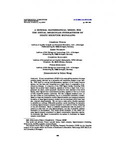
Clearly, x = 0.47 and y = 10%. Therefore, the selling price should be ^2,940 at 10% service charge. Figure (1) shows the graph of x, y against z while figure (2) shows the graph of x, y against F ( x, y ) . The two figures confirm that F ( x, y ) is a correct interpolate of z. Figure (3), below, confirms that the values of x and y are optimal.
350
6. Remark on Results The computed results of problems (1) and (2) reveal that the model for optimizing the sales mark-up price and service charge is accurate and easy to implement.
7. Conclusion Herein, I present this model for optimizing sales mark-up price and service to financial and economic experts who deal with techniques of profit maximization in commerce and industry. Testing the model on real life problems confirm the possibility of obtaining optimal values of sales mark-up price and service charge for a profit-maximizing firm. The obtained results show that the model is amenable to financial analysis and computer automation.
References
Figure 1. Graph of available data points.
[1]
Hall R. L, Hitch C. J. 1952. “Price theory and business behavior,”Oxford economic papers, Oxford University press, pp. 12-46.
[2]
Sylos L. P. 1957. “Oligopoly and technical progress,” Harvard University press, pp. 49-50.
[3]
Colander D. C. 2001. “Microeconomics,”Mcgraw-Hill, New York.
[4]
Sweezy P. 1939. “Demand under conditions of oligopoly,” Journal of political economy (1:1), pp. 568- 737. Koutsoyiannis A. 2003. “Modern microeconomics,” Macmillan press Ltd, India.
[5]
Lewis D. 2014. “How to generate good profit maximization problems,” The journal of Economic Education (45:3), pp. 183-190.
[6]
Daniel A. L., Brian W. U. 2010. “Opportunity costs and nonscale free capabilities: Profit Maximization, Corporate scope and Profit margins”Strategic management journal by Wiley Interscience, (31:1), pp. 780-801.
[7]
Prajit K. D., Radner R. 1999. “Profit maximization and market selection hypothesis,”The review of economic studies, (66:4), pp. 769-798.
[8]
Dutta, P. K. 1994. “Bankruptcy and expected utility maximization,”Journal of Economic Dynamics and control, (18:3), pp. 539-560.
[9]
Radner R. 1998. “Profit maximization withbankcruptcy and variable scale,” Journal of Economic dynamics and control, (22:4), pp. 849-867.
Figure 2. Graph of model (function) data points.
[10] Lau, A. & Lau, H. S. 2003. “Effects of a demand-curve’s shape on the optimal solutions of a multi-echelon inventory/pricing model,” European Journal of Operational Research, (147:3), pp. 530-548. [11] Alchian, A. 1950. “Uncertainty, evolution and economic theory,” Journal of political Economy, (21:3), pp. 39-53.
Figure 3. Contour points of F ( x, y ).
[12] Alfred S. 1975. “Profit maximizing vslabour-managed firms: A comparison of market structure and firm behavior,” The journal of industrial economics, Wiley, (24:2), pp. 97-104.
351 Emmanuel Nwaeze: A Mathematical Model for Optimizing Sales Mark-Up Price and Service Charge in a Profit-Maximizing Firm
[13] Yang, S. L., Zhou, Y. W. 2006. “Two-echelon supply chain models,” International journal of production economics, (103:2), pp. 104-116. [14] Agralwal, N., Smith, S. A., Tsay, A. A. 2002. “Multi-vendor sourcing in a retail supply Chain,”Journal of production and operations management, (11:3), pp. 157-182. [15] Ertek, G., Griffin, P. M. 2002. “Supplier and buyer driven channels in a two stage supply Chain,” IIE Transactions, (34:2), pp. 691-700.
[16] Matrix laboratory (MATLAB). 1984-2007. The Math Works, Inc. [17] Nwaeze, E., Isienyi S. U., Zhengui LI. 2013. “An augmented cubic line search algorithm for solving highdimensionalnonlinear optimization problems,” Journal of the Nigerian mathematical society, (32:3), pp. 185-191.