A Mathematical Programming Model for Tactical ... - RiuNet - UPV

I J

International Journal of Production Management PME and Engineering

doi:10.4995/ijpme.2016.5209 Received 2016-04-06 Accepted: 2016-06-13

A Mathematical Programming Model for Tactical Planning with Set-up Continuity in a Two-stage Ceramic Firm David Pérez Peralesa1, M. M. Eva Alemanya2 a

Research Centre on Production Management and Engineering. Universitat Politècnica de València. a1 a2

[email protected]

[email protected] .

Abstract: It is known that capacity issues in tactical production plans in a hierarchical context are relevant since its inaccurate determination may lead to unrealistic or simply non-feasible plans at the operational level. Semi-continuous industrial processes, such as ceramic ones, often imply large setups and their consideration is crucial for accurate capacity estimation. However, in most of production planning models developed in a hierarchical context at this tactical (aggregated) level, setup changes are not explicitly considered. Their consideration includes not only decisions about lot sizing of production, but also allocation, known as Capacitated Lot Sizing and Loading Problem (CLSLP). However, CLSLP does not account for set-up continuity, specially important in contexts with lengthy and costly set-ups and where product families minimum run length are similar to planning periods. In this work, a mixed integer linear programming (MILP) model for a two stage ceramic firm which accounts for lot sizing and loading decisions including minimum lot-sizes and set-up continuity between two consecutive periods is proposed. Set-up continuity inclusion is modelled just considering which product families are produced at the beginning and at the end of each period of time, and not the complete sequence. The model is solved over a simplified twostage real-case within a Spanish ceramic firm. Obtained results confirm its validity. Key words: Set-up Continuity, Ceramic Firm, Tactical Planning, Mixed Integer Linear Programming.

1. Introduction In the majority of the production planning models developed in a hierarchical context at the tactical level, the capacities at each stage are aggregated and setup changes are not explicitly considered. However, if at this level the setup times involve an important consumption capacity and have been completely ignored, this may lead to an overestimation of the real capacity availability which, in turn, may lead to unrealistic or unfeasible events during the subsequent disaggregation of tactical plans (Pérez, 2013). Considerable savings may be also be achieved through optimum lot-sizing decisions, known in the literature as Capacitated Lot Sizing Problem (CLSP) problem. But standard CLSP does not sequence products within a period and also assumes that setup cost

Creative Commons Attribution-NonCommercial-NoDerivatives 4.0 International https://ojs.upv.es/index.php/IJPME

occur for each lot in a period, even if the last product to be produced in a period is the first one in the period that follows. In addition to that, most of them focus on the operational (disaggregated) level. Many works have addressed the standard CLSP problem such as: Barani et al., 1984; Eppen and Martin, 1987; Chen and Tizy, 1990; Maes et al., 1991; Chung et al., 1994; Hindi, 1996; Belvaux and Wolsey, 2001. Standard CLSP may lead therefore to inaccurated capacity estimations at a tactical (aggregated) level, specially relevant in semicontinuous production environments with lengthy and costly set-ups and where minimum run lengths are similar to planning periods. In these contexts, setup continuity must be incorporated. These models are known as CLSP with setup carryovers or simply CLSP with linked

Int. J. Prod. Manag. Eng. (2016) 4(2), 53-64

53

Pérez Perales, D., Alemany, M.M.E.

lot-sizes (Haase, 1994). These models have not been as intensively studied as the standard CLSP, mainly due to their model complexity and computational difficulty (Sox and Gao, 1999). Just a few works have addressed the CLSP with linked lot-sizes, all of them with constant sequence independent setup times and /or setups, with a setup carryover. No sequence is considered within a period. They just focus on determining the products produced last and first in two consecutive periods, and also the configuration of the machine at the end of the period. Some examples may be found in Kang et al., 1999; Gopalakrishnan et al., 2001; Porkka et al., 2003; Suerie and Stadtler, 2003. But accounting accurately for setup times at the tactical level would mean simultaneously including not only lot sizing decisions, but also allocation of production. This later problem is known as Capacitated Lot Sizing and Loading problem (CLSLP) (Özdamar and Birbil, 1998; Özdamar and Bozyel, 1998). Although the above quoted works consider both allocation and lot sizing issues in a tactical planning level, there is a lack of tactical models in a hierarchical context that consider this CLSLP problem, so that capacities are aggregated and no product families allocation takes place, leading to inaccurate estimation of the real capacity availability that clearly affects to the operational level (Mustafa et al., 1999; Grieco et al., 2001). In addition to that, despite considering product families allocation and lot sizing issues, no setup continuity issues are included, specially in multistage systems. This is particularly important in industrial sectors with semicontinuous processes such as: -- ceramic (Alemany et al., 2009, 2011) -- food (Van Donk, 2001; Soman et al., 2004, 2007; Romsdal et al., 2011; Kopanos et al., 2012a, 2012b). -- textile (Ishikura, 1994; De Toni and Meneghetti, 2000; Guo et al., 2006; Min and Cheng, 2006; Wong and Leung, 2008; Ngaia et al., 2014) -- chemical (Meijboom and Obel, 2007; Ulstein et al., 2007; Teimoury et al., 2010; Fumero et al., 2012; Shabani and Sowlati, 2013; Van Elzzaker et al., 2014) All of them cope with very lengthy setup times in their manufacturing processes and at the same time their product families minimum run length

54


are almost, equal or even higher than the planning period. Many firms in these sectors only work with planning overviews based on spreadsheets. However, given the increasing complexity of product catalogues and current market pressure to reduce supply times, more rigorous methods are needed to optimise resources, as the one mathematical programming-based proposed in this work. Furthermore, given the dramatic increase of end products, the possibilities for assigning and establishing lots on production lines multiply. Therefore, the expected reduction of tactical production planning costs stands out as the proposed model establishes the product families to be produced on each line in an attempt to save changeovers as far as possible, this being an important objective, among others, in the aforementioned sectors. In this article, an approach to accurately model the capacity in tactical (aggregated) plans in a hierarchical context for a ceramic firm is proposed. For that, not only the CLSLP problem is considered, but also setup continuity issues and a two-stage system. Some of this paper authors already approached this issue in Pérez et al. (2014), but in a single stage one. The differences that result from this consideration justify this new scenario. This setup continuity is made over discrete periods of time, that is, it assumes that if a product family is manufactured two periods of time in the same production line just one set-up should be considered. Besides, it accounts for minimum lot sizes even if the product family was produced in a production line in different periods. The set-up continuity consideration along with the minimum lot sizes requirement allows the model to produce the minimum lot-sizes over two consecutive periods being another contribution of the paper. Within this model more efficient and realistic plans will be achieved at the tactical level, reducing later plan modifications due to internal aspects of the firm. The rest of the paper is arranged as follows. Section 2 describes the problem being studied, as is the case of a Spanish ceramic plant. In Section 3, a deterministic MILP model to solve the problem is presented. Section 4 reports a numerical example to validate the model. Section 5 offers some conclusions and future research lines, some of them already being undertaken.

Creative Commons Attribution-NonCommercial-NoDerivatives 4.0 International

A Mathematical Programming Model for Tactical Planning with Set-up Continuity in a Two-stage Ceramic Firm

2. Problem description This case involves a ceramic Spanish plant based in the province of Castellón, dedicated to the manufacture of different types of tiles (floorings and coverings) since 1975. Although this plant forms part of a broader industrial group (tiles SC) which is made up of different plants dedicated to the design, manufacture, marketing and distribution of finished goods, this work is single-company based, and the decisional problem to be addressed just focuses in mid term/tactical production planning issues. Each production plant follows a make-to-stock strategy and it can be classified as a hybrid flow shop composed of several stages (presses-glazing lines, kilns and sorting-packing) uncoupled by buffers .Each stage is integrated by similar machines and different finished goods can be processed by each machine at each stage. The main characteristics of each one of such stages are: 1. Presses-glazing lines: is made up of one or several production lines in parallel with a limited capacity. Production lines may process different product families. Changeovers between product families incur setup costs owing to the time spent in changing, for example, moulds. A product family is defined as a group of finished goods of identical use (flooring or coverings), format (size), grout (white or red), and whose preparation on production lines is similar. This grouping into product families is crucial not only for commercial reasons but also to minimise setup times and costs. Glazing lines may not be standardised, in that case, each product family can be processed according to specific facilities with the appropriate technical features. Therefore, not all glazing lines are capable of processing all the product families, although a product family that may be processed on each line is known. Technological factors involved in the production process mean that when a certain family is manufactured on a specific line, it should be produced in an equal or greater amount than the minimum lot size. This is partly because a certain percentage of defects occur during the production process, and only a percentage of the manufactured items may be sold as first quality finished goods.


2. Kilns: represent the bottleneck section and imply a high energy consumption and cost. Changeovers also occur in this section but are not as important as in the presses-glazing lines. 3. Sorting-packing: this section always has excess capacity and does not represent any critical resource. At the tactical level, an Aggregate Plan (AP) for capacity-related decisions is defined for product families in the first two stages (sorting-packing is not taken into account). In this context not only is important the consideration of setup times but also its continuity over consecutive planning periods, because the set-up are lengthy and the minimum lot sizes of product families imply a run length (3 weeks) similar to the planning periods (1 month). These aspects are crucial to get accurate capacity availability estimation in the AP, which will constraint the master plan.

3. Problem Modeling A MILP model has been developed to solve this ceramic tactical production planning problem. The objective is to minimize the total cost (set-up and inventory) over the time periods of the planning horizon. Decisions will have to simultaneously deal with not only the allocation of product families to production lines and kilns with a limited capacity, but also with the determination of lot sizing and other decisions regard to set-up continuity modelling. For example those which allow to know the first and the last product family processed on each production line and kiln in a planning period, so that one changeover can be saved if the last one processed in t and the first one in t+1 are the same. Or those which allow processing the minimum lot size between two consecutive periods with no changeover. All of them are later explained. The indexes, parameters, and decision variables are described in Tables 1-3, respectively. Table 1. Indexes. f

Product Families (F) (f=1…F)

l

Production Lines (L) (l=1…L)

k

Kilns (K) (k=1….K)

t

Periods of Time (PT) (t=1…T)


55


Table 2. Parameters. dft

Demand of F f in PT t.

cif

Inventory cost of a F f in a PT.

ciif

Inventory cost (intermediate) of a F f in a PT.

cslfl

Setup cost for F f on L l.

cshfk

Setup cost for F f on K k.

tflfl

Time to process a F f on L l.

tfhfk

Time to process a F f on K k.

tslfl

Setup time for F f on L l.

tshfk

Setup time for F f on K k.

lmlfl

Minimum lot size of F f on L l.

lmhfk

Minimum lot size of F f on K k.

capllt

Production capacity available (time) of L l during PT t.

caphkt

Production capacity available (time) of K k during PT t.

i0f

Inventory of F f at the start of the first PT.

ii0f

Inventory (intermediate) of F f at the start of the first PT.

M1,M2,M3,M4

Very large integers.

nf

Number of F

βl0fl

The L l is prepared to produce the F f at the start of the first PT.

βh0fk

The L l is prepared to produce the K k at the start of the first PT.

Table 3. Decision Variables.

56

Ift

Inventory of F f at the end of PT t.

IIft

Inventory (intermediate) of F f at the end of PT t.

PFLflt

Amount of F f produced on L l in PT t.

PFHfkt

Amount of F f produced on K k in PT t.

YLflt

Binary variable with a value of 1 if F f is produced on L l in PT t, and with a value of 0 otherwise.

YHfkt

Binary variable with a value of 1 if F f is produced on K k in PT t, and with a value of 0 otherwise.

XLflt

Binary variable with a value of 1 if L l is ready to produce the F f in PT t, and with a value of 0 otherwise.

XHfkt

Binary variable with a value of 1 if K k is ready to produce the F f in PT t, and with a value of 0 otherwise.

ZLflt

Binary variable with a value of 1 if L l if a setup takes place of F f on L l in PT t, and with a value of 0 otherwise.

ZHfkt

Binary variable with a value of 1 if K k if a setup takes place of F f on K k in PT t, and with a value of 0 otherwise.

WLlt

Binary variable with a value of 1 if more than one F f is produced on L l in PT t, and with a value of 0 otherwise.

WHkt

Binary variable with a value of 1 if more than one F f is produced on K k in PT t, and with a value of 0 otherwise.

αLflt

Binary variable with a value of 1 if L l is prepared to produce the F f at the start of PT t, and with a value of 0 otherwise.

αHfkt

Binary variable with a value of 1 if K k is prepared to produce the F f at the start of PT t, and with a value of 0 otherwise.

βLflt

Binary variable with a value of 1 if L l is prepared to produce the F f at the end of PT t, and with a value of 0 otherwise.

βHfkt

Binary variable with a value of 1 if K k is prepared to produce the F f at the end of PT t, and with a value of 0 otherwise.




Objective Function:

∑∑∑ c sl t

l

f

fl

* ZL flt + ∑∑∑ c sh fh * ZH fht t

h

f

+ ∑∑ c i f * I ft + ∑∑ c i i f * II ft t

f

t

(1)

f

2*XHfkt– αHfkt –βh0fk ≤ 2*ZHfkt, ∀ f, k, t

(20)

∑ ZHfkt ≤ nf *(3– αHfkt– βHfkt –βh0fk), ∀ f, k, t =1

(22)

2*XHfkt– αHfkt –βHfkt–1 ≤ 2*ZHfkt, ∀ f, k, t

(21)

f

Subject to: I ft = i 0 f + ∑ PFH fkt − d ft , ∀ f, t = 1 k

I ft = I ft −1 + ∑ PFH fkt − d ft k

∑ tfh f

fk

∑ tsh f

fk

* PFH fkt + * ZH fkt ≤ caphkt

PFH fkt ≤ M 1* XH fkt PFH fkt ≤ M 2* YH fkt

, ∀ f, t > 1

(3)

, ∀ f, k, t(5) , ∀ f, k, t

(6)

l m h fk *( ZH fkt + ZH fkt +1 + YH fkt +YH fkt +1 − 2) ≤ PFH fkt + PFH fkt +1 YH fkt ≤ PFH fkt , ∀ f, k, t

, ∀ f, k, t

, ∀ f, k, t

YH fkt ≤ XH fkt , ∀ f, k, t ZH fkt ≤ YH fkt , ∀ f, k, t

αHfkt–βh0fk ≤∑ZHfkt, ∀ f, k, t = 1

αHfkt–βHfkt–1 ≤∑ ZHfkt, ∀ f, k, t >1

(7)

(8)

(10) (11) (12) (13)

f

βHfkt–αHfkt ≤(∑ XHfkt)–1, ∀ f, k, t

(14)

f

∑αHfkt=1, ∀ k, t

(15)

f

∑ βHfkt=1, ∀ k, t

(16)

f

αHfkt ≤ XHfkt , ∀ f, k, t βHfkt ≤ XHfkt , ∀ f, k, t

3*XHfkt–∑ XHfkt ≤ αHfkt +βHfkt, ∀ f, k, t

2–∑ YHfkt ≤ 2*(1–WHkt), ∀ k, t

(24)

f

f

fkt

) − 1 ≤ nf *WH kt

, ∀ k, t

αHfkt+βHfkt ≤ (2–WHkt), ∀ f, k, t

(25) (26)

IIft=ii0f +∑ PFLflt – ∑ PFHfkt , ∀ f, t = 1

(27)

IIft= IIft–1 +∑ PFLflt – ∑ PFHfkt , ∀ f, t = 1

(28)

∑ tflfl *PFLflt +∑ tslfl *ZLflt ≤ capllt ∀ l,t

(29)

PFLflt ≤ M 3*XLflt, ∀ f, l, t

(30)

lmlfl*(ZLflt+ZLflt+1–YLflt+1) ≤PFLflt, ∀ l, f, t

(32)

l

k

l

k

l

(9)

(23)

f

(∑ YH

, ∀ k, t(4)

l m h fk *( ZH fkt + ZH fkt +1 − YH fkt +1 ) ≤ PFH fkt

(2)

∑ ZHfkt ≤ nf *(3– αHfkt– βHfkt –βHfkt–1), ∀ f, k, t >1

f

PFLflt ≤ M 4*YLflt, ∀ f, l, t

lmlfl*(ZLflt+ZLflt+1+YLflt+YLflt+1–2)≤PFLflt+PFLflt+1,

∀ l, f, t

(31)

(33)

YLflt ≤ PFLflt , ∀ f, l, t

(34)

ZLflt ≤ YLflt , ∀ f, l, t

(36)

YLflt ≤ XLflt , ∀ f, l, t

(35)

αLflt– βl0fl ≤ ∑ ZLflt , ∀ f, l, t = 1

(37)

f

(17)

αLflt– βLflt–1 ≤ ∑ ZLflt , ∀ f, l, t >1

(38)

f

(18)

βLflt– αLflt ≤ (∑ XLflt )–1, ∀ f, l, t

(39)

f

(19)

f


∑ αLflt=1, ∀ l, t

(40)

f


57


∑ βLflt=1, ∀ l, t

(41)

βLflt ≤ XLflt , ∀ f, l, t

(43)

f

αLflt ≤ XLflt , ∀ f, l, t

(42)

3*XLflt–∑ XLflt ≤ αLflt+ βLflt , ∀ f, l, t

(44)

2*XLflt– αLflt+ βLflt–1 ≤ 2*ZLflt , ∀ f, l, t

(46)

f

2*XLflt– αLflt+ βl0fl ≤ 2*ZLflt , ∀ f, l, t

(45)

∑ ZLflt ≤ nf *(3–αLflt–βLflt–βl0fl) , ∀ f, l, t = 1

(47)

f

∑ ZLflt ≤ nf *(3–αLflt–βLflt–βLflt–1) , , ∀ f, l, t > 1

(48)

Constraint (9) establishes that if there is no amount of F produced on a K in a PT then it is not allowed to produce the F on the K in such a PT. Constraint (10) establishes that if a F is produced on a K in a PT, then the K has been previously prepared to produce the F in such a PT. Constraint (11) establishes that if a F is not produced on a K in a PT, then there is no setup on the K in such a PT. Constraints (12) and (13) ensure that if a K “status” at the start of a PT is different from the “status” at the end of the previous PT, then at least one setup has to be made on the K in such a PT. Constraint (14) indicates that if a K does not change its “status” during a PT, then it is already prepared (either at the start or the end of such a PT) to produce the same F.

f

2–∑ YLflt ≤ 2 *(1–WLlt), ∀ l, t

(49)

f

(∑ ZLflt )–1≤ nf *WLlt, ∀ l, t

(50)

f

αLflt+ βLflt ≤(2–WLlt), ∀ f, l, t

(51)

The objective function (1) expresses the minimization of the setup costs of the Fs on the Ls and Ks (both stages) and the inventory costs of the Fs at the middle (intermediate) and the end of the manufacturing process. Constraints (2) and (3) are the inventory balance equations of in-process and finished Fs, respectively. Constraint (4) ensures that the capacity required for the setup of Fs and the manufacturing of the lots assigned to each K do not exceed the capacity available on each K in each PT. Constraint (5) indicates that a F can only be produced on a K in a PT if the K has previously be prepared to produce the F in such a PT. Constraint (6) indicates that a F can only be produced on a K in a PT if it has previously been decided to produce the F on the K in such a PT. Constraint (7) guarantees that should a certain amount of a F be produced on a K, it is equal to or above the minimum lot size established for the F on that K if the F is just produced in a single PT. Constraint (8) allows not to produce the minimum lot size established for a F on a K in a PT, if either the F was the last one produced in the previous PT and the first one produced in the next PT, or the F is the only one produced during two consecutive PTs. However, it guarantees in both cases that the total amount of F produced will be superior to its minimum lot size.

58


Constraints (15) and (16) guarantee that a K can be only prepared to produce just one F, in the start and in the end of a PT, respectively. Constraints (17) and (18) ensures that if a K is not prepared to produce a F in a PT, then that F can not be either the first or the last, respectively, for which the K was prepared in such a PT. Constraint (19) indicates that if a K is only prepared to produce just one F in a PT, then the K should be prepared either at the start or the end of such a PT to produce the F. Constraints (20) and (21) indicate that it is only possible to save a single changeover on a K in a PT if the K is prepared at the start of the current PT to manufacture the same F for which it was prepared at the end of the previous PT. Constraints (22) and (23) indicate that if the “status” of a K at the start and the end of a current PT is equal to the “status” at the end of the previous PT, then just one or no F is manufactured. Constraint (24) assures that if one or no F is manufactured on a K in a PT, then WL=0, although the contrary case does not imply WL=1. For this it is implemented constraint (25). Constraint (26) guarantees that if more than one F is manufactured on a K in a PT, none of them can be the first and the last at the same time in such a PT. Therefore, only in the case in which one or no F is manufactured on a K in a PT is possible that αH=1 and βH=1 for that F. Constraints (27) and (28) are the inventory balance equations of intermediate products (between Ls and Ks). Constraints from (29) to (51) are the same as constraints from (4) to (26) but in this case regarding to the Ls.



4. Numerical example The model validation is made by its application to a simplified two-stage real case within a ceramic firm. The input data and the solution obtained are described in the following sections.

4.1. Input data description The model data are based on historical information (demand data) and on the mean real values (times and costs). The physical configuration has been slightly changed for confidentiality reasons, considering a problem of a size that represents the main relevant characteristics, but not excessively large so that it could be described in detail here. The model’s planning horizon is assumed to be half a year and it is divided into six monthly planification periods, from t1 to t6. Six product families labelled F1 to F4 were included, each of them corresponding to different formats. Only a single plant is considered, made up of two stages. First one, presses-glazing lines stage consists of three production lines , from L1 to L3. Second one, kilns stage, consists of two kilns, K1 and K2. Both stages are uncoupled by buffers.

In addition to the former table, some specific data of product families on production lines and kilns are shown in Table 5. No backorder is permitted. The proposed model was translated to the MPL language, V4.2. The resolution was carried out with optimisation solver GUROBI 4.5.1. The input data and the model solution values were processed with the Microsoft Access database (2007). The experiment was run on a PC with a 2.40 GHz processor and 2 GB of RAM. Table 5. Specific data of product families (F) in each of the production lines (L) and kilns (K). i0

ciif

tslf

cslf

tflf

lmlf

βl0lf

F1

F

L

50

0.1

2

35

0.1

160

0

F2

50

0.15

2.5

30

0.25

180

1

F3

50

0.2

3

40

0.2

175

0

F4

50

0.15

3.5

45

0.2

160

0

F5

50

0.25

2.5

30

0.1

180

0

F6

50

0.1

3

45

0.15

170

0

F1

50

0.1

2

35

0.1

160

0

F2

50

0.15

2.5

30

0.25

180

0

F3

50

0.2

3

40

0.2

175

1

F4

50

0.15

3.5

45

0.2

160

0

F5

50

0.25

2.5

30

0.1

180

0

F6

50

0.1

3

45

0.15

170

0

F1

50

0.1

2

35

0.1

160

1

F2

50

0.15

2.5

30

0.25

180

0

F3

50

0.2

3

40

0.2

175

0

F4

50

0.15

3.5

45

0.2

160

0

F5

50

0.25

2.5

30

0.1

180

0

F6

50

0.1

3

45

0.15

170

0

cif

tshf

cshf

tfhf

lmhf

βh0kf

L1

L2

L3

Other relevant FGs data for the model can be consulted in Tables 4-5. Data of product families demand, and production capacity in each of the production lines (L) and kilns in each period of time are shown in Table 4.

F

K

ii0

F1

50

0.1

10

120

1.5

160

0

F2

50

0.15

15

115

1.8

180

1

F3

50

0.2

18

100

2.5

175

0

F4

50

0.15

16

125

2

160

0

F5

50

0.25

15

110

3.5

180

0

F6

50

0.1

17

100

1.5

170

0

F1

50

0.1

10

120

1.5

160

0

F2

50

0.15

15

115

1.8

180

0

F3

50

0.2

18

100

2.5

175

1

F4

50

0.15

16

125

2

160

0

F5

50

0.25

15

110

3.5

180

0

F6

50

0.1

17

100

1.5

170

0

K1

Table 4. Data of product families (F) demand and production capacity of production lines (L) and kilns (K) in each PT (t). F F1

d ft t1

t2

t3

t4

t5

t6

100

125

135

140

150

130

F2

125

110

135

150

125

115

F3

140

125

110

130

115

125

F4

100

125

135

140

150

130

F5

125

110

135

150

125

115

F6

140

125

110

130

115

125

L

capl lt t1

t2

t3

t4

t5

t6

L1

50

70

70

50

70

70

L2

70

50

70

50

50

70

L3

50

50

50

70

70

50

K

caph kt t1

t2

t3

t4

t5

t6

K1

1000

1250

1000

1000

1200

1200

K2

1200

1100

1100

1200

1300

1000


K2

4.2. Evaluation of results The values of the decision variables linked to the production lines and kilns that lead to the optimum solution and help to validate the set-up continuity are shown in Tables 6-9.


59


Table 6. Amount (m2) of product families (F) manufactured on production lines L1 and L2 in each PT. t1 L1

PFL

XL

YL

βl0=F2 ZL

L2

PFL

XL

YL

βl0=F3 ZL

F1 F2 F3 F4 F5 F6 F1 F2 F3 F4 F5 F6 F1 F2 F3 F4 F5 F6 αL βL F1 F2 F3 F4 F5 F6 WL

F1 F2 F3 F4 F5 F6 F1 F2 F3 F4 F5 F6 F1 F2 F3 F4 F5 F6 ALFAL BETAL F1 F2 F3 F4 F5 F6 WL

t2

164

40

t4

t3 230

465

t6

115

125

1 1

1

1

XL

YL

βl0=F1 ZL

60

F1 F2 F3 F4 F5 F6 F1 F2 F3 F4 F5 F6 F1 F2 F3 F4 F5 F6 αL βL F1 F2 F3 F4 F5 F6 WL

F1 F2 F3 F4 F5 F6 F1 F2 F3 F4 F5 F6 F1 F2 F3 F4 F5 F6 αH βH F1 F2 F3 F4 F5 F6 WH

1 YH

1

1

1

1

1 βh0=F2

1 F2 F6

1 F6 F6

1 F3 F6

F3 F3

F3 F3

ZH

F3 F3

1 K2

1 1

1

175 125

35

140

350

170

1 1

1

1

125

1

1

F3 F4

F4 F4

F4 F4

F4 F1 1

YH

1

1 1

115

1

1

1

βh0=F3

1

1

F1 F5

F5 F5

1

1

1

1

t2

260

25

185

1

1

t4

t5

106

150

240

1

1

1

1

1

1

1

1

F5 F5

F5 F2

1

1

F2 F2

F2 F2

1 1 1


185

1

t4

t5

t6

122

150

240 115

125

1

1 1

1

1

1 1

1

F2 F2

F2 F3

F3 F3

210 1

1 1

1

1

1 1

1 1

1

1

F2 F5

F5 F5

F5 F2 1

1

1 1 1

1

225

230 135

310

90 1

465

1 1

1 1 F6 F6

125

1

1

1

F4 F1 1

1 1 1 1

1

1

1

1 F6 F4

115

1

1

1 1 1

1 F3 F6 1

280

420

140 1 1

1 1

1

140

1

1

F1 F5

F5 F5

1

1

1

1

F

IIft

Ift

t1

t2

t3

t4

t5

t6

t1

t2

t3

t4

t5

t6

F1

0

0

0

0

0

0

260

135

0

0

130

0

F2

16

16

0

0

0

0

123

13

0

0

115

0

F3

0

0

0

0

0

0

135

10

130

0

0

0

F4

0

35

250

0

0

0

125

0

0

280

130

0

F5

0

0

0

0

0

0

0

75

150

0

0

0

F6

0

0

0

0

0

0

0

340

370

240

125

0

1

1

F1 F5

1

t6

210 1

175 75

t3

Table 9. Intermediate and final inventory of product families (F) at each PT (t).

1

t3

ZH

t2

198

F1 F2 F3 F4 F5 F6 F1 F2 F3 F4 F5 F6 F1 F2 F3 F4 F5 F6 αH βH F1 F2 F3 F4 F5 F6 WH

XH

1

1 1

PFH

280

1

t1 PFL

PFH

XH

Table 7. Amount (m2) of product families (F) manufactured on production line L3 in each PT.

L3

t1 K1

140

1

1

t5

Table 8. Amount (m2) of product families(F)manufactured on kilns K1 and K2 in each PT.

F2 F2

The assessment method used consisted in analyzing if the model accounts for set-up continuity issues. However, the model operation was also assessed by two parameters: computational efficiency and the total costs in terms of tactical planning. These results confirm that the described constraints are valid to model the set-up continuity over discrete periods of time. It implies that if a product family is manufactured in two periods of time just one set-up is considered. This occurs just in case F is the last to be manufactured on a L or a K in a PT t and the first Creative Commons Attribution-NonCommercial-NoDerivatives 4.0 International


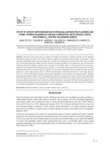
to be manufactured on the same L or K in PT t+1. In addition to that, the model allows the minimum lot size may be completed without any changeover during these two consecutive periods. A representative example may be seen in Table 6 for F1, which is manufactured on L2 in two consecutive PTs t=4 and t=5. F1 is manufactured at the end of PT t=4 in an amount less than its minimum lot size although it is also manufactured at the start of PT t=5, therefore meeting that minimum lot size of 160 and just considering one set-up instead of two. Another example may be seen in Table 8 for F4, which is manufactured on K2 in two consecutive PTs t=3 and t=4. F4 is manufactured at the end of PT t=3 in an amount less than its minimum lot size although it is also manufactured at the start of PT t=4, therefore meeting that minimum lot size of 160 and just considering one set-up instead of two. In Table 10 , the values of the total costs are shown. This paper focuses on the validation of set-up continuity issues so that some simplifications in the example are assumed, leading to approximated results of the reality. As aforementioned, tactical production planning in real ceramic SC scenarios includes a wide variety of production mix and other additional variables/costs, mainly related with the number of shifts planned in the press-glazing lines, the activation / desactivation of kilns or the subcontracting of some supplementary capacity for certain products families. In our example, the model generated a total cost of € 1894.4. The different components of the objective function appear in Table 10: intermediate and final inventory costs and setup costs in both stages. Backorder costs are not reflected in the model assuming that all the demand has to be fulfilled. Finally, problem size characteristics and computational efficiency can be consulted in Table 11. Table 10. Total Costs.

Table 11. Computational efficiency. Computational efficiency Iterations

133745292

Variables

1182

Integers

1182

Constraints Non-zero Density (%) Time (hours) MIP best bound

2922 12804 0.4 30 1437.15

The computational efficiency parameter measures the computational effort required to solve models. The indicators are: the number of iterations needed by the solver and used to reach the final solution. Table 11 shows the number of model variables, the number of integers in the model, the number of constraints in the model, the number of non-zero elements in the constraints matrix that the model contains, the density of the constraints matrix that the model contains, the CPU time required to obtain the model solution and the MIP best bound. In this case, the model was solved by the standard solver setting the parameter “limit time” to 30 hours, obtaining a gap of 20% regarding to the optimal solution (Table 11). More efficient solutions could be reached, applying other solution techniques. For instance, from the validation of the model, the authors have observed that the solution time of the model substantially decreases by fixing the value of the binary variables YLfltand YHfkt. Therefore, the development of heuristics or metaheuristics similar to Motta et.al (2013) that evaluate different solutions generated by fixing the value of the binary variables YLflt and YHfkt, transferring them as input data to the model and optimize the value of the remaining decision variables, could substantially reduce the solution time and the gap. However, this issue is out of scope of this work and constitutes a future research line.

Total Costs Intermediate Inventory costs Final Inventory costs Press-glazing Lines Set-up costs Kilns Set-up costs

47.55 389.15 255 1125 1816.7


5. Conclusions This work presents a mix integer linear programming (MILP) model to solve the tactical planning problem in a two stage production system in the ceramic sector for the purpose of minimizing product families


61


set-up and inventory costs, while considering set-up continuity and a given forecasted mid-term demand. The model contemplated was validated by a ceramic real-world case example, but one on a smaller scale for the purpose of providing details of all the input data and of the solution obtained, focusing on product families allocation and set-up continuity aspects. Although it is just considered a two-stage production process, it might be adapted to larger models for specific situations replicating the links between the additional stages and extrapolated to other semi-continuous production sectors. Its main contributions are on one hand the accounting for explicit setup times at the tactical (aggregated) level which implies including decisions about the product families allocation and lot sizing of production. On the other hand the consideration of set-up continuity constraints, especially important in contexts with lengthy set-ups and where product

families minimum run length are almost, equal or even higher than the planning period. The set up continuity modelling also allows the consideration of minimum lot sizes produced during two consecutive periods. Both contributions help to achieve a more accurate capacity availability estimation in the tactical level so it may lead to feasible and more efficient events during the subsequent disaggregation into operational plas. The model has been validated by its application to a realistic ceramic firm. The obtained results confirm that the proposed model accounts for both issues: product families allocation and set-up continuity. For larger real problems with more time periods and/or products it should be necessary to develop solution techniques to reduce the computational time. For this reason, future research lines could develop efficient solution methods by means heuristic or metaheuristics applied to this problem.

References Alemany, M.M., Alarcón, F., Lario, F.C., Boj, J.J. (2009). Planificación agregada en cadenas de suministro del sector cerámico. III internacional conference on industrial engineering and industrial management. Barcelona, Spain 3-42. Alemany, M.M., Boj, J.J., Mula, J., Lario, F.C. (2011). Mathematical programming model for centralised master planning in ceramic tile supply chains. International Journal of Production Research, 48, 5053-5074. http://dx.doi.org/10.1080/00207540903055701 Barany, I., Van Roy, T.J., Wolsey, L.A. (1984). Strong formulations for multi-item capacitated lot sizing. Management Science, 30(10), 1255–1261. http://dx.doi.org/10.1287/mnsc.30.10.1255 Belvaux, G., Wolsey, L.A. (2001). Modelling practical lot-sizing problems as mixed-integer programs. Management Science, 47(7), 724-38. http://dx.doi.org/10.1287/mnsc.47.7.993.9800 Chen, W.H., Thizy, J.M. (1990). Analysis of relaxations for the multi-item capacitated lot-sizing problem. Annals of Operations Research, 26, 29-72. http://dx.doi.org/10.1007/BF02248584 Chung, C., Flynn, J., Lin, C.M. (1994). An efective algorithm for the capacitated single item lot size problem. European Journal of Operational Research, 75(2), 427-40. http://dx.doi.org/10.1016/0377-2217(94)90086-8 De Toni, A., Meneghetti, A. (2000).The production planning process for a network of firms in the textile-apparel industry. International Journal of Production Economics, 65(1), 17-32. http://dx.doi.org/10.1016/S0925-5273(99)00087-0 Eppen, G.D., Martin, R.K. (1987). Solving multi-item capacitated lot sizing problems using variable redefinition. Operations Research, 35(6), 832–48. http://dx.doi.org/10.1287/opre.35.6.832 Fumero, Y., Montagna, J.M., Corsano, G. (2012). Simultaneous design and scheduling of a semicontinuous/batch plant for ethanol and derivatives production. Article Computers & Chemical Engineering, 36, 342-357. http://dx.doi.org/10.1016/j. compchemeng.2011.08.004 Gopalakrishnan, M., Ding, K., Bourjolly, J.M., Mohan, S. (2001). A tabu-search heuristic for the capacitated lot-sizing problem with set-up carryover. Management Science, 47(6), 851–863. http://dx.doi.org/10.1287/mnsc.47.6.851.9813 Grieco, S., Quirico, S., Tullio, T. (2001). A Review of Different Approaches to the FMS Loading Problem. International Journal of Flexible Manufacturing Systems, 13(4), 361-384. http://dx.doi.org/10.1023/A:1012290630540 Guo, Z.X., Wong, W.K., Leung, S.Y.S., Fan, J.T., Chan, S.F. (2006). Mathematical model and genetic optimization for the job shop scheduling problem in a mixed- and multi-product assembly environment: A case study based on the apparel industry. Computers & Industrial Engineering, 50(3), 202-219. http://dx.doi.org/10.1016/j.cie.2006.03.003 Haase, K. (1994). Lotsizing and scheduling for Production Planning. In: Lecture Notes in Economics and Mathematical Systems. SpringerVerlag, Berlin. http://dx.doi.org/10.1007/978-3-642-45735-7

62




Hindi, K.S. (1996) .Solving the CLSP by a tabu search heuristic. Journal of the Operational Research Society, 47(1), 151–61. http://dx.doi. org/10.1057/jors.1996.13 Ishikura, H. (1994). Study on the production planning of apparel products: Determining optimal production times and quantities. Computers & Industrial Engineering, 27(1/4), 19-22- http://dx.doi.org/10.1016/0360-8352(94)90227-5 Kang, S., Malik, K., Thomas, L.J. (1999). Lotsizing and scheduling on parallel machines with sequence dependent setup costs. Management Science, 45(2), 273-289. http://dx.doi.org/10.1287/mnsc.45.2.273 Karacapilidis, N., Pappis, C. (1996). Production planning and control in textile industry: A case study. Computers in Industry, 30(2), 127-144. http://dx.doi.org/10.1016/0166-3615(96)00038-3 Kopanos, G.M., Puigjaner, L., Georgiadis, M.C. (2012a). Simultaneous production and logistics operations planning in semicontinuous food industries. Omega, 40(5), 634-650. http://dx.doi.org/10.1016/j.omega.2011.12.002 Kopanos, G.M., Puigjaner, L., Georgiadis, M.C. (2012b). Single and multi-site production and distribution planning in food processing industries. Computer Aided Chemical Engineering, 31, 1030-1034. http://dx.doi.org/10.1016/B978-0-444-59506-5.50037-7 Maes, J., McClain, J.O., Van Wassenhove, L.N. (1991). Multilevel capacitated lot sizing complexity and LP-based heuristics. European Journal of Operational Research, 53(2), 131-48. http://dx.doi.org/10.1016/0377-2217(91)90130-N Newson, E.F. (1975). Multi-item lot size scheduling by heuristic, part I: with fixed resources. Management Science, 21(10), 1186-1193. http://dx.doi.org/10.1287/mnsc.21.10.1086 Meijboom, B., Obel, B. (2007). Tactical coordination in a multi-location and multi-stage operations structure: A model and a pharmaceutical company case. Omega, 35(3), 258-273. http://dx.doi.org/10.1016/j.omega.2005.06.003 Min, L., Cheng, W. (2006). Genetic algorithms for the optimal common due date assignment and the optimal scheduling policy in parallel machine earliness/tardiness scheduling problems. Robotics and Computer-Integrated Manufacturing, 22(4), 279-287. http://dx.doi. org/10.1016/j.rcim.2004.12.005 Motta C.F., Resendo R., Morelato P. (2013). A hybrid multi-population genetic algorithm applied to solve the multi-level capacitated lot sizing problem with backlogging, Computers & Operations Research, 40 910–919. http://dx.doi.org/10.1016/j.cor.2012.11.002 Mustafa, K., Sinan, K., Nesim, E. (1999). A Generic Model to Solve Tactical Planning Problems in Flexible Manufacturing Systems. International Journal of Flexible Manufacturing Systems, 11(3), 215-243. http://dx.doi.org/10.1023/A:1008182411581 Ngaia, E.W.T., Penga, S., Alexander, P., Moon, K. (2014). Decision support and intelligent systems in the textile and apparel supply chain: An academic review of research articles. Expert Systems with Applications, 41(1), 81-91. http://dx.doi.org/10.1016/j.eswa.2013.07.013 Özdamar, L., Birbil, S.I. (1998). Hybrid Heuristics for the capacitated lot sizing and loading problem with setup times and overtime decisions. European Journal of Operational Research,110(3), 525-547. http://dx.doi.org/10.1016/S0377-2217(97)00269-5 Özdamar, L., Bozyel, A. (1998).Simultaneous lot sizing and loading of product families on parallel facilities of different classes. International Journal of Production Research, 36(5), 1305-1324. http://dx.doi.org/10.1080/002075498193336 Romsdal, A., Thomassen, M.K., Dreyer, H.C., Strandhagen, J.O. (2011). Fresh food supply chains; characteristics and supply chain requirements. 18th international annual EurOMA conference. Cambridge, UK, Cambridge University. Pérez, D. (2013). Framework and methodology proposal for the modeling of the supply chain collaborative planning process based on mathematical programming. Application to the ceramic sector. Dissertation, Universitat Politècnica de València Pérez, D., Alemany M.M.E., Lario, F.C., Fuertes, V.S. (2014).Set-up Continuity in Tactical Planning of Semi-Continuous Industrial Processes. Managing Complexity. Springer International Publishing, 165-173. Porkka, P., Vepsalainen, A.P.J., Kuula, M. (2003). Multiperiod production planning carrying over set-up time. International Journal of Production Research, 41(6), 1133–1148. http://dx.doi.org/10.1080/0020754021000042995 Shabani, N., Sowlati, T. (2013). A mixed integer non-linear programming model for tactical value chain optimization of a wood biomass power plant. Applied Energy, 104, 353-361. http://dx.doi.org/10.1016/j.apenergy.2012.11.013 Soman, C.A., Van Donk, D.P., Gaalman, G.J.C. (2004). Combined make-to-order and make-to-stock in a food production system. International Journal of Production Economics, 90(2), 223–235. http://dx.doi.org/10.1016/S0925-5273(02)00376-6 Soman, C.A., Van Donk, D.P., Gaalman, G.J.C. (2007). Capacitated planning and scheduling for combined make-to-order and make-tostock production in the food industry: An illustrative case study. International Journal of Production Economics, 108(1-2), 191–199. http://dx.doi.org/10.1016/j.ijpe.2006.12.042 Sox, C.R., Gao, Y.B. (1999). The capacitated lot sizing problem with setup carry-over. IIE Transactions, 31(2), 173–181. http://dx.doi. org/10.1080/07408179908969816 Suerie, C., Stadtler, H. (2003). The capacitated lot-sizing problem with linked lot sizes. Management Science, 49(8), 1039–1054. http:// dx.doi.org/10.1287/mnsc.49.8.1039.16406 Teimoury, E., Modarres, M., Ghasemzadeh, F., Fathi, M. (2010). A queueing approach to production-inventory planning for supply chain with uncertain demands: Case study of PAKSHOO Chemicals Company. Journal of Manufacturing Systems, 29(2/3), 55-62. http://dx.doi. org/10.1016/j.jmsy.2010.08.003



63


Ulstein, N.L., Nygreen, B., Sagli, J.R. (2007). Tactical planning of offshore petroleum production. European Journal of Operational Research, 176(1), 550-564. http://dx.doi.org/10.1016/j.ejor.2005.06.060 Van Donk, D.P. (2001). Make to stock or make to order: The decoupling point in the food processing industries. International. Journal of Production Economics, 69(3), 297–306. http://dx.doi.org/10.1016/S0925-5273(00)00035-9 Van Elzakker, M.A.H., Zondervan, E., Raikar, N.B., Hoogland, H., Grossmann, I.E. (2014). An SKU decomposition algorithm for the tactical planning in the FMCG industry. Computers & Chemical Engineering, 62(5), 80-95. http://dx.doi.org/10.1016/j.compchemeng.2013.11.008 Wong, W.K., Leung, S.Y.S. (2008). Genetic optimization of fabric utilization in apparel manufacturing. International Journal of Production Economics, 114(1), 376-387. http://dx.doi.org/10.1016/j.ijpe.2008.02.012

64

