Oct 5, 2010 - best way to teach PLC controlled process, allowing project testing in an ... used to implement the PLC control program in Matlab/Simulink ...
A Matlab/Simulink Framework for PLC Controlled Processes
211
11 X
A Matlab/Simulink framework for PLC controlled processes João Martins and Celson Lima
CTS, UNINOVA, Departamento de Engenharia Electrotécnica, Faculdade de Ciências e Tecnologia, Universidade Nova de Lisboa Portugal
Herminio Martínez and Antoni Grau
College of Industrial Engineering of Barcelona (EUETIB), U.E. d’Electrònica Industrial Technical University of Catalonia (UPC) Spain 1. Introduction Relevant literature recognises that the practical test of an automation and control process controlled by programmable logic controllers (PLC) is a well-known problem [1-3]. There are several solutions that can be implemented, such as scale models, batteries of led’s and switches and Human Machine Interfaces (HMI), Supervisory Control and Data Acquisition (SCADA) systems, or simulation tools. The use of scale models of real processes is very expensive and difficult to adapt to different processes. There is no question that this is the best way to teach PLC controlled process, allowing project testing in an almost real environment, however their cost often prohibits its use. The use of leds and switches sets is extremely confusing end uninteresting. This approach, only valid when small processes are considered, severely reduces the motivation. Some HMI and SCADA systems allow this feature but there are very expensive, not intended for this purpose and usually consider property protocols. The use of Matlab®/Simulink® [4] has not been a regular approach for teaching industrial automation and PLC controlled processes. Assuming that the model of the industrial process is implemented in the Matlab/Simulink, this chapter presents a tool that can be used to implement the PLC control program in Matlab/Simulink environment. The basic idea is to consider the PLC control program as a Matlab function block, within the Matlab/Simulink environment, that will control the model of the industrial process as long as the simulation runs. The main objective of the work described in this chapter is to automatically translate the PLC control program, written as an instruction list, into Matlab/Simulink software language.
www.intechopen.com
212
Matlab - Modelling, Programming and Simulations
2. State-of-the-art Although programmable logic controllers (PLC) have many definitions, one can affirm that they are solid-state members of the computer family, using integrated circuits instead of electromechanical devices to implement control functions. They can be thought of in simple terms as industrial computers with specially designed architecture in both their central units (the PLC brain) and their input/output (I/O) interfacing circuitry with the real world. PLCs are capable of storing instructions, such as sequencing, timing, counting, logic, arithmetic, data manipulation, and communication, to control industrial machines and processes [5]. Fig. 1 shows a conceptual diagram of a PLC application.
Process or machine
Control signals or actions
Measure signals
Field outputs
Programmable Logic Controller (PLC)
Field inputs
Fig. 1. Conceptual diagram of a PLC application. The Hydramatic Division of the General Motors Corporation specified the design criteria for the first programmable controller in 1968. Their primary goal was to eliminate the high costs associated with inflexible, relay controlled systems. The specifications required a solid-state system with computer flexibility to survey in an industrial environment, be easily programmable and maintained by plant engineers and technicians, and be reusable. The first PLC had its first product models in 1969. These early controllers met the original specifications and opened the doors to the development of a new control technology. PLCs provided an easy way to reprogram the wiring rather than actually rewiring the control system. The first PLCs offered relay functionality, thus replacing the original hardwired relay logic. Notice that they were more or less just relay replacers: Their primary functions were to perform the sequential operations that were previously implemented with relays (ON/OFF control of machines and processes that required repetitive operations, such as transfer lines and grinding and boring machines). However, the first programmable controllers were a vast improvement over relays: They were easily installed, used considerably less space and energy, had diagnostic indicators that aided troubleshooting, and unlike relays, were reusable if a project should be modified. 2.1 Today’s Programmable Logic Controllers Many technological advances in the programmable controller industry continue today. These advances not only affect programmable controller design, but also the philosophical approach to control system architecture and programming. In fact, changes include both hardware (physical components) and software (control program) upgrades. Thus, the following list describes some recent PLC hardware enhancements:
www.intechopen.com
A Matlab/Simulink Framework for PLC Controlled Processes
213
Faster scan times are being achieved using new, advanced microprocessor and electronic technology. Small, low-cost PLCs, which can replace four to ten relays, now have more power than their predecessor, the simple relay replacer. High-density input/output (I/O) systems provide space-efficient interfaces at low cost. Intelligent, microprocessor-based I/O interfaces have expanded distributed processing. Typical interfaces include PID (proportional-integral-derivative) controllers, network, CANbus, fieldbus, ASCII communication, positioning, host computer, and language modules (e.g., BASIC, Pascal). Mechanical design improvements have included rugged input/output enclosures and input/output systems that have made the terminal an integral unit. Special interfaces have allowed certain devices to be connected directly to the controller. Typical interfaces include thermocouples, strain gauges, and fastresponse inputs. Peripheral equipment has improved operator interface techniques, and system documentation is now a standard part of the system. All of these hardware enhancements have led to the development of programmable controller families. These families consist of a product line that ranges from very small “microcontrollers,” with as few as 10 I/O points, to very large and sophisticated PLCs, with as many as 8000 I/O points and 128000 words of memory. These family members, using common I/O systems and programming peripherals, can interface to a local communication network. The family concept is an important cost-saving development for users. Like hardware advances, software advances, such as the ones listed below, have led to more powerful PLCs: PLCs have incorporated object-oriented programming tools and multiple languages based on the IEC 1131-3 standard. Small PLCs have been provided with powerful instructions, which extend the area of application for these small controllers. High-level languages, such as BASIC and C, have been implemented in some controllers’ modules to provide greater programming flexibility when communicating with peripheral devices and manipulating data. Advanced functional block instructions have been implemented for ladder diagram instruction sets to provide enhanced software capability using simple programming commands. Diagnostics and fault detection have been expanded from simple system diagnostics, which diagnose controller malfunctions, to include machine diagnostics, which diagnose failures or malfunctions of the controlled machine or process. Floating-point math has made it possible to perform complex calculations in control applications that require gauging, balancing, and statistical computation. Data handling and manipulation instructions have been improved and simplified to accommodate complex control and data acquisition applications that involve storage, tracking, and retrieval of large amounts of data.
www.intechopen.com
214
Matlab - Modelling, Programming and Simulations
Programmable controllers are now mature control systems offering many more capabilities than were ever anticipated. They are capable of communicating with other control systems, providing production reports, scheduling production, and diagnosing their own failures and those of the machine or process. These enhancements have made programmable controllers important contributors in meeting today’s demands for higher quality and productivity. Despite the fact that programmable controllers have become much more sophisticated, they still retain the simplicity and ease of operation that was intended in their original design. 2.2 Programmable Logic Controllers and the Future The future of programmable controllers relies not only on the continuation of new product developments, but also on the integration of PLCs with other control and factory management equipment. PLCs are being incorporated, through networks, into computerintegrated manufacturing (CIM) systems, combining their power and resources with numerical controls, robots, CAD/CAM systems, PCs, management information systems, and hierarchical computer-based systems. There is no doubt that programmable controllers will play a substantial role in the factory of the future. New advances in PLC technology include features such as graphic user interfaces (GUIs), better operator interface (human-machine interfaces or HMIs), and more human-oriented man/machine interfaces (such as voice modules). They also include the development of interfaces that allow communication with equipment, hardware, and software that supports artificial intelligence, such as fuzzy logic controllers, etc. 2.3 Mechanical Configurations for PLC Systems There are four common types of mechanical design for PLC systems: Single-board PLCs or open frame PLCs. Compact PLCs or single-box PLCs (sometimes referred to as a brick PLCs or shoebox PLCs). Semi-modularized PLCs. Modularized PLCs, modular PLCs or rack types. On the one hand, single board PLCs are basic PLCs available on a single printed circuit board. They are totally self-contained (normally with the exception of a power supply) and, when installed in a system, they are simply mounted inside a control cabinet on threaded standoffs [6]. Single board PLCs are very inexpensive, easy to program, small, and consume little power, but, generally speaking, they do not have a large number of inputs and outputs, and have a somewhat limited instruction set. They are best suited to small, relatively simple control applications. On the other hand, PLCs are also available housed in a single case with all input and output, power and control connection points located on the single unit. In this case, they are known as compact PLCs. This kind of programmable controllers is generally chosen according to available program memory and required number and voltage of inputs and outputs to suit the application. The compact type is commonly used for small programmable controllers and is supplied as an integral compact package complete with power supply, processor, memory, and input/output units. Typically such a PLC might have 6, 8, 12, or 24 inputs and 4, 8, or 16 outputs and a memory that can store some 300 to 1000 instructions.
www.intechopen.com
A Matlab/Simulink Framework for PLC Controlled Processes
215
Some compact systems have the capacity to be extended to cope with more inputs and outputs by linking input/output boxes to them. This kind of PLCs is known as semimodularized units [7].These systems generally have an expansion port (an interconnection socket) which will allow the addition of specialized units such as high speed counters and analog input and output units or additional discrete inputs or outputs. These expansion units are either plugged directly into the main case or connected to it with ribbon cable or other suitable cable. Finally, systems with larger numbers of inputs and outputs and more sophisticated units, with a wider array of options, are likely to be modular and designed to fit in racks (modularized PLCs) [8]. The modular type consists of separate modules for power supply, processor, and the like, which are often mounted on rails within a metal cabinet. The rack type can be used for all sizes of programmable controllers and has the various functional units packaged in individual modules that can be plugged into sockets in a base rack. The mix of modules required for a particular purpose is decided by the user and the appropriate ones then plugged into the rack. Thus it is comparatively easy to expand the number of I/O connections by simply adding more input/output modules or to expand the memory by adding more memory units. The power and data interfaces for modules in a rack are provided by copper conductors in the backplane of the rack. When modules are slid into a rack, they engage with connectors in the backplane. 2.4 Scopes of Applications and Sizes for PLC Systems Prior to evaluating the system requirements, the designer should understand the different ranges of programmable controller products and the typical features found within each range. This understanding will enable the designer to quickly identify the type of product that comes closest to matching the requirements of the application. Fig. 2 illustrates PLC product ranges divided into five major areas with overlapping boundaries. The basis for this product segmentation is the number of possible inputs and outputs the system can accommodate (I/O count), the amount of memory available for the application program, and the general hardware and software of the system structure. As the I/O count increases, the complexity and cost of the system also increase. Similarly, as the system complexity increases, the memory capacity, variety of I/O modules, and capabilities of the instruction set increase as well. Thus, PLC market or their scopes of applications can be segmented into five groups [5]: Micro PLCs. Small PLCs. Medium PLCs. Large PLCs. Very large PLCs.
www.intechopen.com
216
Matlab - Modelling, Programming and Simulations
Complexity and cost
5 Area 1: Micro PLCs Area 2: Small PLCs Area 3: Medium PLCs Area 4: Large PLCs Area 5: Very Large PLCs
C 4 B 3 A 2 1
I/O Count 32
64
128 512 1024 2048 4096
8192
Fig. 2. PLC product ranges. The shaded areas in Fig. 2, labeled A, B, and C, reflect the possibility of controllers with enhanced (not standard) features for a particular range. These enhancements place the product in a shady area that overlaps the next higher range. For example, because of its I/O count, a small PLC would fall into area 2, but it could have analog control functions that are standard in medium-sized controllers. Thus, this type of product would belong in area A. Products that fall into these overlapping areas allow the user to select the product that best matches the requirements of his/her application, without having to select the larger product, unless it is necessary. Thus, micro PLCs are used in applications controlling up to 32 input and output devices, 20 or less I/O being the norm. The micros are followed by the small PLC category, which controls 32 to 128 I/O. The medium (64 to 1024 I/O), large (512 to 4096 I/O), and very large (2048 to 8192 I/O) PLCs complete the segmentation. In particular, micro PLCs (area 1) are used in applications that require the control of a few discrete I/O devices, such as domotic applications and small conveyor controls. Some micro PLCs can perform limited analog I/O monitoring functions (e.g., monitoring a temperature set point or activating an output). Small PLCs (area 2) are mostly used in applications that require ON/OFF control for logic sequencing and timing functions. These PLCs, along with microcontrollers, are widely used for the individual control of small machines. Often, these products are single-board controllers. In addition, area A includes controllers that are capable of having up to 64 or 128 I/O, along with products that have features normally found in medium-sized controllers. The enhanced capabilities of these small controllers allow them to be used effectively in applications that need only a small number of I/O, yet require analog control, basic math, I/O bus network interfaces, LANs, remote I/O, and/or limited data-handling capabilities. A typical application of an area A controller is a transfer line in which several small machines, under individual control, must be interlocked through a LAN. Medium PLCs (area 3) are used in applications that require more than 128 I/O, as well as analog control, data manipulation, and arithmetic capabilities. In general, the controllers in segment 3 have more flexible hardware and software features than the controllers
www.intechopen.com
A Matlab/Simulink Framework for PLC Controlled Processes
217
previously mentioned. Area B contains medium PLCs that have more memory, table handling, PID, and subroutine capabilities than typical medium-sized PLCs, as well as more arithmetic and data-handling instructions. Large PLCs (area 4) are used for more complicated control tasks, which require extensive data manipulation, data acquisition, and reporting. Further software enhancements allow these products to perform complex numerical computations. Area C includes the segment 4 PLCs that have a large amount of application memory and I/O capacity. The PLCs in this area also have greater math and data-handling capabilities than other large PLCs. Very large PLCs (area 5) are used in sophisticated control and data acquisition applications that require large memory and I/O capacities. Remote and special I/O interfaces are also standard requirements for this type of controller. Typical applications for very large PLCs include steel mills and refineries. These PLCs usually serve as supervisory controllers in large, distributed control applications. 2.5 PLC Architecture The typical blocks for a general programmable controller are [6]: The processor, the mounting rack, the input and output modules, the power supply and the programming unit. The processor (also known as CPU), as in the self contained units, is generally specified according to memory required for the program to be implemented. The processor consists of the microprocessor, system memory, serial communication ports for printer, PLC LAN link and external programming device and, in some cases, the system power supply to power the processor and I/O modules. Notice that, in modularized versions, capability can also be a factor. This includes features such as higher math functions, PID control loops and optional programming commands. The mounting rack is usually a metal framework with a printed circuit board backplane which provides means for mounting the PLC input/output (I/O) modules and processor. Mounting racks are specified according to the number of modules required to implement the system. The mounting rack provides data and power connections to the processor and modules via the backplane. For CPUs that do not contain a power supply, the rack also holds the modular power supply. There are systems in which the processor is mounted separately and connected by cable to the rack. The mounting rack can be available to mount directly to a panel or can be installed in a standard equipment cabinet. Mounting racks are “cascadable” so several may be interconnected to allow a system to accommodate a large number of I/O modules. The input and output (I/O) modules are specified according to the input and output signals associated with the particular application. These modules fall into the categories of discrete, analog, high speed counter or register types. Discrete I/O modules are generally capable of handling 8 or 16 and, in some cases 32, on-off type inputs or outputs per module. Modules are specified as input or output but generally not both although some manufacturers now offer modules that can be configured with both input and output points in the same unit. The module can be specified as AC only, DC only or AC/DC along with the voltage values for which it is designed. Analog input and output modules are available and are specified according to the desired resolution and voltage or current range. As with discrete modules, these are generally input or output; however some manufacturers provide analog input and output in the same module. Analog modules are also available which can directly accept thermocouple inputs for temperature measurement and monitoring by the PLC. Pulsed
www.intechopen.com
218
Matlab - Modelling, Programming and Simulations
inputs to the PLC can be accepted using a high speed counter module. This module can be capable of measuring the frequency of an input signal from a tachometer or other frequency generating device. These modules can also count the incoming pulses if desired. Generally, both frequency and count are available from the same module at the same time if both are required in the application. Register input and output modules transfer 8 or 16 bit words of information to and from the PLC. These words are generally numbers (BCD or Binary) which are generated from thumbwheel switches or encoder systems for input or data to be output to a display device by the PLC. Other types of modules may be available depending upon the manufacturer of the PLC and its capabilities. These include specialized communication modules to allow for the transfer of information from one controller to another. The power supply specified depends upon the manufacturer's PLC being utilized in the application. As stated above, in some cases a power supply capable of delivering all required power for the system is furnished as part of the processor module. If the power supply is a separate module, it must be capable of delivering a current greater than the sum of all the currents needed by the other modules. For systems with the power supply inside the CPU module, there may be some modules in the system which require excessive power not available from the processor either because of voltage or current requirements that can only be achieved through the addition of a second power source. This is generally true if analog or external communication modules are present since these require ± DC supplies which, in the case of analog modules, must be well regulated. The programming unit allows the engineer or technician to enter and edit the program to be executed. In its simplest form it can be a hand held device with a keypad for program entry and a display device (LED or LCD) for viewing program steps or functions. More advanced systems employ a separate personal computer which allows the programmer to write, view, edit and download the program to the PLC. This is accomplished with proprietary software available from the PLC manufacturer. This software also allows the programmer or engineer to monitor the PLC as it is running the program. With this monitoring system, such things as internal coils, registers, timers and other items not visible externally can be monitored to determine proper operation. Also, internal register data can be altered if required to fine tune program operation. This can be advantageous when debugging the program. Communication with the programmable controller with this system is via a cable connected to a special programming port on the controller. Connection to the personal computer can be through a serial port or from a dedicated card installed in the computer.
3. Industrial Process Modeling and Simulation 3.1 Why Modeling? In order to study, analyze and control systems, it is necessary to know them very well and, thus, to have a mathematical model that describes them. This model can be used in a computer simulator tool (as MATLAB/Simulink), or for the analysis and design purposes of control systems. On the one hand, in case a model is developed for a computer simulator, in general, such a model will be represented in a complex and complete way in order to describe as accurate and realistic as possible the real system behavior. On the other, in case a control is needed for the analysis or design purposes of a control system, a representation of this model will be required in its simplest manner, but always taking into account the essence of the model
www.intechopen.com
A Matlab/Simulink Framework for PLC Controlled Processes
219
and its more characteristic behavior. Therefore, the goal in modeling techniques is to achieve models in a simple or complex manner depending on the application and objectives. In this Section, we will briefly focus on the development of control models that describe industrial processes that will be useful to controllers’ tuning. Models serve to represent and determine systems behavior and thus fulfill at least three purposes: Prediction, learning new rules and/or data compression. Models can be developed in two different ways or two basic approaches. Let us imagine in the need, in the other hand quite often, of crossing a closed door without knowing the direction of opening. A possibility to know the right direction of opening is to observe the arrangement of hinges; this would be a theoretical approach. The other possibility is to try to open the door choosing one of the directions; this would be the experimental approach. Following, there is the definition of both approaches: Theoretical approach: This approach consists of building a model from physical laws. Here, the engineer can find the difficulty of managing all the physical laws that take part, and in case the model is achieved, it could be very complex and thus difficult to manage. Moreover, another drawback of this approach is that real phenomena are not taken into account such as components wearing, tolerances, noise and disturbance effects… Experimental approach or identification: When a system is not suitable for the theoretical approach due to many reasons (such as its complexity, an incomplete knowledge of the system structure or due to an unpredictable variation of its features), it is necessary to resort to another approach that permits the achievement of valid and suitable models. This second approach consists of analyzing the system based on the study of its output signals in front of a well-known set of input signals. In this approach, to not adopt any hypothesis about the system’s characteristics usually makes the study difficult, limiting its quality. The experience demonstrates that the best solution is the combination of both approaches, whenever it is possible. In this case, two steps are usually carried out: The analysis stage and, then, the experimental stage. In the analysis stage, physical laws and work conditions (operation modes) will be taken into account in order to establish the hypothesis. In the experimental stage, starting from the hypothesis set in the analysis, the obtained experimental measures will be considered to determine the coefficients of the mathematical model. In order to obtain the system’s response, it is necessary to stimulate it thanks to the input variables that are generated from the environment of the system under study. There exist two kinds of system input variables: Those that can be controlled, and those that cannot be controlled and are automatically generated by the environment (known as disturbances, Fig. 3). The variables generated by the system are the output variables and they influence on the environment. Those variables are measurable and, sometimes, observable. Suppose a system like the presented one in Fig. 3. Mainly, two problems can arise with this system: Direct problem or analysis: knowing (input, system), find (output). This problem has a unique solution and it is called a problem of analysis. Inverse problems: o Knowing (input, output), find (system). This problem does not have a unique solution but it has infinite correct solutions. This is a problem of
www.intechopen.com
220
Matlab - Modelling, Programming and Simulations
o
structure identification and state estimation, and it is called a problem of synthesis. Knowing (system, output), find (input). This is a problem of control (instrumentation).
Fig. 3. System Diagram. 3.2 Modelling and simulation spectrum A system can belong to different disciplines, and each one presents different aspects that should be taken into account when treating this system. The modeler can face a kind of systems that present only historical data, for instance, public opinion systems or social areas systems (see Fig. 4). Models can only be built from experimentation and the modeling technique is identification that is mainly used when the system structure is unknown. In this case, the models are call black box models, and they can be represented with differential equations. In the real world, there exist many complex systems which evolution depends on various variables (time, space…) and the most suitable way to describe them is through Partial Differential Equations (PDEs) because they are systems with distributed parameters. In the field of Environmental Sciences is where those systems can be mainly found (Ecology, pollution, biodiversity…). The models developed in these systems are mostly for prediction and experimentation of management strategies. Finally, there is another kind of systems that their physical laws are perfectly known, that is, the system structure is known and they can be built using white box models. From those models the differential equations are generated and, in the most of the cases, they are straightforward enough to be represented with Ordinary Differential Equations (ODEs) because normally their parameters are concentrated. For instance, electric and electronics circuits, chemical control processes, industrial control and aerospatial systems can be represented with white box models. In these cases, the obtained models are used to design a controller to manage the process. As it can be seen in Fig. 4, from the black box models to white box models there are all the models that a modeler can find in the real world.
www.intechopen.com
A Matlab/Simulink Framework for PLC Controlled Processes
221
Fig. 4. Modeling: from white box to black box. 3.3 Mathematical model representation Linear Time-Invariant (LTI) systems are represented by ODEs, but these expressions are too much complicated to manipulate. Thus, modelers use equivalent and easier expressions to represent these equations, for instance, Laplace transform. This representation permits to obtain the transfer function describing the system, mainly used in SISO (Single Input Single Output) systems. An alternative to represent a system is through the state space representation, mainly used in MIMO (Multiple Input Multiple Output) systems. The main feature of state space representation is that the internal system variables are represented (all the system’s stated) whereas the transfer function only represents the relationship between output and input of the system. In control engineering, a state space representation is a mathematical model of a physical system as a set of input, output and state variables related by first-order differential equations. To abstract from the number of inputs, outputs and states, the variables are expressed as vectors and the differential and algebraic equations are written in matrix form (the last one can be done when the dynamical system is linear and time invariant). The state space representation (also known as the "time-domain approach") provides a convenient and compact way to model and analyze systems with multiple inputs and outputs. With p inputs and q outputs, we would otherwise have to write down q x p Laplace transforms to encode all the information about a system. Unlike the frequency domain approach, the use of the state space representation is not limited to systems with linear components and zero initial conditions. "State space" refers to the space whose axes are the state variables. The state of the system can be represented as a vector within that space.
www.intechopen.com
222
Matlab - Modelling, Programming and Simulations
3.4 Steps for the simulation project To choose the type of model to apply is important to know the objectives for which the model will be used. After chosen the model that best fits to the objectives, the system model is developed using the physical laws and/or identification, depending on the situation. Then, the model has to be implemented and validated using obtained real data (data base). To validate the model any error criterion is used, and if the model has goodness enough the process is over, in opposite case the model is reconsidered and the selection process starts again looking for the model that best fits with the system and all the process is repeated until we are satisfied with the chosen model. The whole process can be seen in Fig. 5.
Fig. 5. Simulation steps. 3.5 Simulation Software Mathematical modeling and simulation are emerging as key technologies in engineering. Relevant computerized tools, suitable for integration with traditional design methods are essential to meet future needs of efficient engineering. Interactive simulation provides a flexible and user-friendly method to define the experiments performed on the model. During the interactive simulation run, the user can change the values of the model inputs (signals of interest or disturbances), system parameters and initial conditions of the state variables, perceiving instantly how these changes affect to the model dynamic. As a consequence, interactive simulation facilitates the development and improvement of the model performance and allows enhancing the understanding of the system behavior. This capability is especially useful when the model is being used for educational purposes [9]. 3.5.1 Today’s simulation tools There is a large amount of simulation software on the market. All languages and model representations are proprietary and developed certain tools. There are general-purpose tools such as ACSL, MATLAB-Simulink, and System Build. They are based on the same modeling methodology, input-output blocks, as in the previous standardization effort, CSSL, from
www.intechopen.com
A Matlab/Simulink Framework for PLC Controlled Processes
223
1967. There are domain-oriented packages: electronic programs SPice, Saber, Multibody Systems, HADAMS, DADS, SIMPACKI, chemical processes (ASPEN Plus, SpeedUp), etc. In October 1996, an international effort started to design a new language for physical modeling. The language is called Modelica. The main objective is to make it easy to exchange models and model libraries and to allow users to benefit from the advances in object oriented modeling methodology [10]. On the other hand, there exists novel simulation software, for instance Easy Java Simulations (Ejs), that lastly is growing and widely used because it is a freeware, open source, Java-based tool intended to create interactive dynamic simulations [11]. Ejs was originally designed to be used by students for interactive learning, under the supervision of educators with a low programming level. As a consequence, simplicity was a requirement. Ejs guides the user in the process of creating interactive simulations. This process includes the definition of the model and the view. The use of Ejs, together with Matlab/Simulink and Modelica/Dymola allows us to combine the best features of each tool. Ejs has the capability for building interactive user-interfaces composed of graphical elements, whose properties are linked to the model variables. Matlab/Simulink has the capability for modeling of automatic control systems and for model analysis. Modelica has the capability for physical modeling, and finally Dymola has the capability for simulating hybrid-DAE (differential-algebraic equations) models. It is important to highlight that, with a few exceptions, all simulation packages are only strong in one domain and are not capable of modeling components in other domains reasonably. This is a major disadvantage since technical systems are becoming more and more heterogeneous with components from many engineering domains. JMAG provides state of the art technology to encompass extensive physical phenomena accurately in the simulation model. JMAG's precise analysis supports superior electromechanical design. In addition, Spice, in its different versions (PSpice, HSpice, etc.), is the main simulation software in the field of Electronics and Electrical Engineering. PSIM is another simulation package specifically designed for power electronics and motor control. Finally, apart from the industrial process software simulation software, there exists another line of simulators: The PLC simulator. In this field, developers can find software packages such as PC-SIM, a good option for PLC programming learning, because it has a very good graphical environment, among other features. Another tool is SIMTSX, a software package that enables debugging some PLC commercials brands without the presence of the machine or process and allows validate PLC programs and associated control command functions, and training for control and maintenance operators before taking charge of the equipment on site. Some PC-based process simulation tools have been developed, using microcontroller technologies and designed to work with any type of PLC [12]. The PLC modeling issue can be reduced to the emulation of the PLC control program and many approaches can be further taken regarding the PLC program. Several authors developed specific packages for the verification of the PLC program [13,14]. These packages verify the structure of the program using, among others, automata networks. Often these programs only verify the program structure without verifying if it achieves the desired control objectives. Other approach is the generation of the PLC program from other formalisms, such as Petri nets [15], state diagrams, or finite state machines. If the original formalism is error free this could be a valuable tool for developing PLC programs. Some authors developed software
www.intechopen.com
224
Matlab - Modelling, Programming and Simulations
packages to translate PLC programs to DSP code, so that it can be used in non-PLC hardware [16]. None of these approaches is intended to be used within the Matlab/Simulink environment. The proposed methodology approach will consider that the PLC is essentially modelled by emulating its control program, which interacts with the controlled industrial process itself, as presented in Fig. 1.
4. PLC/Matlab Translation Methodology In order to fully understand the advantages of the proposed translation methodology, let us assume that the industrial process is already modelled in the Matlab/Simulink environment, as presented in Fig. 6.
Fig. 6. PLC operation and Industrial Process interaction The industrial PLC controlled process is simulated in a Matlab/Simulink block named ‘Industrial Process Simulation Block’. This block outputs (sensors and detectors outputs) are the process sensors and detectors signals, which will be used as inputs to the Matlab/Simulink block named ‘PLC Control Program’. This block will emulate the PLC operation and its outputs will correspond to the PLC outputs that will connect to the actuators input, in the ‘Industrial Process Simulation Block’. The block ‘PLC Control Program’ is the keystone of the proposed methodology. It will emulate the cyclic PLC operation. This function block is a Matlab m-file. In order to automatically build this block, the following procedures must be accomplished: 1. Assume a PLC-controlled process, which is already modelled in an already existing ‘Industrial Process Simulation Block’, developed in Matlab/Simulink environment; 2. Consider the functional specifications of this PLC-controlled process; 3. Consider a specific PLC to control the process; 4. Elaborate the respective PLC control program accordingly to the considered functional specifications, using for example the GRAFCET methodology [17]; 5. Write down the PLC control program using one of the vendor’s programming languages;
www.intechopen.com
A Matlab/Simulink Framework for PLC Controlled Processes
225
6. Save the PLC control program as a text-oriented programming language in a text file; 7. Run the developed PLC–Matlab/Simulink translation package in order to convert the PLC control program into the Matlab/Simulink language (the Matlab/Simulink m-file function block ‘PLC control program’ should be automatically produced); 8. Test the developed PLC control program with the considered PLC-controlled process model (Matlab/Simulink m-file function block ‘Industrial Process Simulation Block’); 9. Elaborate the required adaptations in order to put the program control to work properly. The proposed PLC–Matlab/Simulink translation package, before automatically translate the PLC control program into Matlab/Simulink language, will require the following information: 1. Type of PLC; 2. PLC’s number of inputs and outputs; 3. PLC control program file for translation. 4.1 Type of PLC The choice of the PLC type is essential for establishing the translation rules accordingly to the manufacturer program syntax. Although they are all boolean logic based, each PLC manufacturer develops its own programming syntax. In this way the translation package should know the PLC manufacturer in order to apply the adequate translation rules. 4.2 PLC’s number of Inputs and outputs The number of PLC’s Inputs and Outputs clearly defines the arguments of the Matlab/Simulink function ‘PLC Control Program’ (1). This function will be responsible for executing the PLC control program within the Matlab/Simulink environment, and will be created as a text m-file. Both di1 to din denote the PLC’s digital inputs, ai1 to aim denote the PLC’s analog inputs, do1 to dop denote the PLC’s digital outputs and ao1 to aoq denote the PLC’s analog outputs. n, m, p and q denote, respectively, the PLC’s number of digital inputs, analog inputs, digital outputs and analog outputs. It is important to note that n+m define the dimension of the Mux block (a) in Fig. 6. Similarly p+q define the dimension of the Demux block (b) in Fig. 6.
function output
PLC Control Program di1 ,..., din ,..., ai1 ,..., aim
...
PLC Control Pr ogram in Matlab / Simulink language ...
output do1 ,..., dop ,..., ao1 ,..., aoq
www.intechopen.com
(1)
226
Matlab - Modelling, Programming and Simulations
4.3 PLC Control Program file for translation The PLC control program can be written in a wide set of programming languages. The software model of PLC’s and the referred set of languages are established and defined in the IEC standard 1131-3. Every manufacturer offers different kinds of suitable programming languages, resulting in a typical set of five programming languages: Instruction List: Very close to assembler can be considered as a low-level text programming language; Ladder Diagrams: Historically derived from electric circuits wiring does not allow complexity and modularity; Sequential Functional Chart: A Petri Net like graphical programming language it structures the internal elements of the PLC into steps (associated with actions) and transitions (between steps); Function Block Diagram: Another graphical language where function blocks process the several PLC’s signals; Structured Text: Derived from Pascal programming language, it is a high level programming language that enables complexity and modularity. The PLC control program is typically represented using a graphical language known as a ladder diagram. However, almost every PLC software-programming packages allows the use of text-oriented programming languages. Moreover, they allow the automatic conversion between ladder diagrams and text-oriented programming languages, and viceversa. The proposed translation methodology will consider that the PLC control program is written as a text-oriented programming language, in a standard text file. This does not represent a problem because, as referred, almost every PLC software-programming package allows saving the PLC control program in this format. Fig 7 shows a simple PLC Control Program text file considering, as an example, a Siemens PLC. 1 2 3 4 5 6 7 8 9 10 11 12 13 14 15 16 17
// // PROGRAM TITLE COMMENTS // NETWORK 1 LD I 0.0 A I 0.1 LD I 0.2 A I 0.3 OLD = Q 0.0 // NETWORK 2 LD I 0.4 LD I 0.5 CTU C5,+6 // END
Fig. 7. PLC Control Program standard text file The PLC control program translation package is a software tool, developed in Visual Basic, which automatically converts the PLC control program text file into a correspondent Matalb/Simulink m-file. This m-file, containing the PLC control program described in Matalb/Simulink language, holds the Matalb/Simulink function defined in (1). Knowing
www.intechopen.com
A Matlab/Simulink Framework for PLC Controlled Processes
227
the PLC’s number of inputs/outputs, the conversion tool establishes the correct number of input and output arguments for function (1). The translation of the PLC Control Program itself relays on a set of translation rules applied to the set of PLC instruction list. A full PLC instruction list can be roughly divided into: Boolean Comparison Output Timer Counter Math Increment/Decrement Moving/Shifting Program Control Other Following some instructions conversion rules will be described, considering a Siemens PLC instruction list. Boolean instructions will be translated into Matlab/Simulink language using standard Matlab boolean functions, as presented in Table 1, where I x.y denotes a digital input and Q x.y denotes a digital output, x and y are, respectively, the byte and bit of the considered digital input/output. Furthermore, do_g is a Matlab variable denoting digital output g and di_h is a Matlab variable denoting the digital input h. The bollean state TRUE will be represented in Matalb environment by ‘1’ and FALSE by ‘0’. Combinations of various Boolean instructions will be converted using the above rules. An example is shown on the last row of Table 1. Boolean instruction
PLC instruction
Matlab/Simulink translation
AND
LD I a.b A I c.d = Q e.f
do_g = di_h&di_i
OR
LD I a.b O I c.d = Q e.f
do_g = di_h | di_i
NOT
Combinations of various Boolean instructions
LDN I a.b = Q c.d LD I 0.0 A I 0.1 LD I 0.2 OLD = Q 0.0
do_g = ~ di_i
do_1 = (di_1 & di_2) | di_3
Table 1. Boolean Instructions Translation PLC math instructions are usually boolean enabled. This implies the use of Matlab function ‘if’ in order to represent their behavior. As an example, consider the PLC integer adding instruction presented in Table 2. AIW0 and AQW0 represent, respectively, a PLC analog input and a PLC analog output. Variable ao_1 is a Matlab variable denoting the first analog output and ai_1 is a Matlab variable denoting the first analog input.
www.intechopen.com
228
Matlab - Modelling, Programming and Simulations
On n the other hand,, PLC control pro ograms often use internal flags (bit and variable in nternal meemories) to repreesent states or to store analog vallues. Whenever tthe translation paackage fin nds a PLC internaal memory, autom matically assigns a Matlab/Simuliink variable to it. These varriables are usuallly denoted as m or v, as they arre digital or analog. The PLC mu ultiply insstruction (MUL) often involves th he use of an auxiiliary internal meemory, as presen nted in Taable 2, where the MOVW M instructio on (moving the value v of one word d variable – 16 bitt – into another) is also used. Please, note th hat the PLC intern nal variable VD reefers to a 32-bit word. w Instructtion INCREM MENT
MULTIP PLY
PLC C instruction 0 LD I 0.0 +I AIW W0 , AQW0 LD I 0.0 0 MOV VW +6 , VD4 MUL +9 , VD4
Matlab/Simulin nk translation
if di_1 ao_1 = ai_1 + ao_1 end if di_1 v_4 = +6 v_4 = +9 * v_44 end
Table 2. Non-Booleaan Instructions Translation T PL LC counter instru uctions (CTUD – counter up an nd down) can reequire several bo oolean inp puts: One for cou unting up, other for counting dow wn (if the case) aand other for ressenting thee counter. Since the t counting is only o performed on o the rising edge of the boolean input, thee Matlab/Simulin nk translation sho ould take into account the previou us state of that bo oolean inp put. Table 3 preseents a counting example, where di_1_prev is a Mattlabb variable denoting thee previous state of variable di_11. Previous state means the statee in the previou us PLC Co ontrol Program Cycle. C In this example, by reachin ng counting 4 thee counter boolean n state chaanges to true. In n Matlab environm ment c_10 denotees the boolean sttate of counter number 10,, and c_10_value denotes the coun nting value of the same counter. PL LC timer instructiions, such as on--delay timers, usu ually require onlly one digital inp put for cou unting. As Fig. 8 presents, the on n-delay timer (T3 33 in the examplee) works whenev ver the resspective digital in nput (I2.0 in the example) e is enableed, and becomes Boolean TRUE when w it reaaches its preset tim me (3 seconds in the example).
Fig g. 8. On-delay tim mer operation Th he previous timeer translation is presented in Ta able 3. Wheneveer the timer starrts (its corrresponding digiital input – di_200 –is TRUE and the t timer has nott started yet) the preset tim me (t33_start) is added a to the actu ual clock value (cllock_in) establish hing the timer sto opping tim me (t33_end_timee). After reaching this stopping tim me the logical vallue of the timer (tt1_bin) beccomes true. The timer t is restarted when its corresp ponding boolean iinput becomes FA ALSE.
www.intechopen.com
A Matlab/Simulink Framework for PLC Controlled Processes Instruction
COUNTER
TIMER
PLC instruction
LD LD LD CTUD
I 0.0 // Count up I 0.1 // Count down I 0.2 // Reset counter C10, +4
LD I 2.0 TON T33, 3
229 Matlab/Simulink translation
if di_1 & ~ di_1_prev c_10_value = c_10_value + 1 end if di_2 & ~ di_2 c_10_value = c_10_value - 1 end if di_3 c_10_value = 0 c_10 = 0 end if c_10_value >= +4 c_10 = 1 end
%Start timer if di_20 & t33_start==0 t33_start=3; t33_end_time=clock_in+3; end %Timer ON if t33_start &clock_in>=t33_end_time t33_bin=1; end %Timer OFF if ~di_20 t33_bin=0; t33_start=0; end
Table 3. Counter and Timer Instructions Translation
5. Application Examples As a first illustrative application example let us consider pure Boolean. It is supposed to automate the sawmill presented on Fig. 9. After pressing the START pushbutton the cutting machine moves to the right. The blade must be connected before it reaches the logs and cut off after sawing them. At this time the blade should be raised. When the top position is reached the upward movement should stop and the machine must move to the left until it reaches its original position, where the blade should be lowered. In Fig. 9 are also depicted the limit switches (denoted as Si) that are used to control the machine actions.
www.intechopen.com
230
Matlab - Modelling, Programming and Simulations
Fig g. 9. Sawmill macchine he PLC’s list of the process inputs and outputs. It shows each signal Taable 4 presents th description, its PLC C address and th he corresponding g Matlab/Simulin nk assignment. For this a 5 digital outp puts are required d. A standard SIEMENS automated process 6 digital inputs and nd 6 digital outpu uts is considered to perform the desired d S7--200 PLC with 8 digital inputs an pro ocess control. Thee process control algorithm was elaborated accordingly to the GRA AFCET, (Graphe Fonctionn nel de Commande Étape Transitio on) or SFC (Sequ uential Function Chart) preesented in Fig. 100. Signaal description
PLC I/O address
Notes
Matlab/ Simulink assignment
Start
I 0.0
Pu ush button
di0
Switch on saw s position
I 0.1
Lim mit switch – S1
di2
Switch off saw s position
I 0.2
Lim mit switch – S2
di3
Machine lo owered
I 0.3
Lim mit switch – S3
di4
Machine raaised
I 0.4
Lim mit switch – S4
di5
Machine att start position
I 0.5
Lim mit switch – S5
di6
Left displaccement
Q 0.0
Mo otor M1 - left
do1
Right displlacement
Q 0.1
Mo otor M1 - right
do2
Saw rotatin ng
Q 0.2
Mo otor M2
do3
Raise mach hine
Q 0.3
Mo otor M3 - up
do4
Lower macchine
Q 0.4
Mo otor M3 - donw
do5
Table 4. Boolean Insstructions Translaation om this GRAFCE ET the PLC control program is written w as a text-oriented program mming Fro lan nguage, in a stand dard text file. Ap pplying the develo oped PLC–Matlaab/Simulink transslation package to this textt file, it automaticcally produces thee Matlab/Simulin nk m-file function n block LC control progrram’. The type of PLC and the number n of I/O w were also consideered as ‘PL traanslation processs package argum ments. The obtain ned m-file, contaaining the PLC control c pro ogram written in n Matalb/Simulin nk language, hollds the Matalb/S Simulink version of the developed control program. It is prresented in (2), where w mi denotees each GRAFCE ET step and mi_a its previo ous boolean valuee.
www.intechopen.com
A Matlab/Simulink Framework for PLC Controlled Processes
231
Fig g. 10. Sawmill GR RAFCET ffunction [ [output]=cpu222( (di1,di2,di3,di4,dii5,di6,di7,di8,ai1,,ai2,ai3,ai4,clock__in ) g global m0 m0_a m1 m m1_a m2 m2_aa m3 m3_a m4 m4_a m m5 m5_a %output initializaation % a aux=0; do1=aux; do2=aux; d do3=au ux; do4=aux; do5= =aux; do6=aux; a ao1=aux; ao2=aux x; ao3=aux; ao4=aaux; %grafcet step evo % olution m m0=(m5&di3)|(m m0&~m5); m m1=(m0&di1&di6 6&di4)|(m1&~m m0); m m2=(m1&di2)|(m m2&~m1); m m3=(m2&di3)|(m m3&~m2); m m4=(m3&di5)|(m m4&~m3); m m5=(m5&di6)|(m m5&~m4); %Output generation % d do1=m1; d do2=m2; d do3=m3; d do0=m4; d d04=m5; %grafcet previouss steps actualization % m m0_a=m0; m m1_a=m1; m m2_a=m2; m m3_a=m3; m m4_a=m4; m m_a=m5; o output=[do1 do2 do3 do4 do5 do66 ao1 ao2 ao3 ao4]];
www.intechopen.com
(2)
232
Matlab - Modelling, Programming and Simulations
Th he second examplle (including timeer and counter op perations) consid ders a water tank with a ran ndom flow of inp put water, whose level should be kept k between 4 an nd 5 meters heigh ht (Fig. 11)). In order to acccomplish this go oal an electric ou utput valve (with h 8 l/sec flow rate) r is con ntrolled by a PLC C. The PLC contro ols this valve acco ordingly to the in nformation provid ded by tw wo level detectors (installed at 4 an nd 5 meter heightt respectively). In n this example it is also desired to count th he number of times that the ou utput valve is acctuated. Wheneveer this umber reaches 8, two t types of alarm ms should be pro oduced: A light siignal and a buzzeer. The nu bu uzzer, however, should s only be activated one seecond after the ccounter has reached 8. Ad dditionally, for testing purposes, an a external reset signal s is considered at 3 and 12 secconds.
g. 11. Water tank level control Fig g. 12 presents th he Matlab/Simulink environmen nt for this appliccation. The subssystem Fig “W Water Tank System m” contains the simulated s model of the water tank k, with its detecto ors and acttuators. The subsytem “PLC” conttains the Matlab/ /Simulink version n of the developeed PLC pro ogram control. Actually A this subsystem simulatess the PLC action n over the processs. The PL LC inputs are: “Maximum “ water level switch”, “Minimum watter level switch””, and “External counter reset”. The two first inputs are the signals prov vided by the two o level k. The PLC outputs are: “Output valve”, “Counteer=8?”, detectors installed in the water tank Counter Alarm” and a “Valve coun nter”. This last output o is an anaalogue output wiith the “C nu umber of times thaat the output valv ve has been opera ated. Th he chosen PLC fo or this application n was again a SIIEMENS S7-200 w with 8 digital inp puts, 4 analog inputs, 6 digital d outputs and a 4 analog ou utputs. This auto omatically defin nes the nu umber and type of o input and outp put arguments off the Matlab/Sim mulink subsystem m “PLC Co ontrol Program”. The input argu uments are the SIEMENS S S7-200 inputs and the clock, wh hile the subsystem m output argumeents are the SIEM MENS S7-200 outp puts. Table 5 defin nes the PL LC’s data and thee respective repreesentation in thee Matlab/Simulin nk environment, where thee description of each data variablee is also presented d.
www.intechopen.com
A Matlab/Simulink Framework for PLC Controlled Processes
233
Fig g. 12. Matlab/Sim mulink model of the t controlled water tank system Signal descrip ption
PLC signall
Notes
Matlaab/ Simulink assignm ment
Maximum level
I 0.0
Switch
di11
Minimum level
I 0.1
Switch
di22
External counter reset
I 0.2
Pushbutton n
di33
Valve
Q0.0
Electric valv ve
do11
Light signal alarm
Q0.0
Signals 8 va alve operations
do22
Q0.2
One second d delay after light sig gnal
do33
Counter vallue
ao11
Buzzer signal alarm m Counter value
QW100
Valve operation cou unter
C1
Internal cou unter (CTU)
Counter alarm timeer
T1
Internal tim mer (on-delay)
c1 t1
GRAFCET1 step 0
M10.00
Internal ma ark
m00
GRAFCET1 step 1
M10.11
Internal ma ark
m11
GRAFCET1 step 2
M10.22
Internal ma ark
m22
GRAFCET 2 step 0
M20.00
Internal ma ark
m100
GRAFCET 2 step 1
M20.11
Internal ma ark
m111
Table 5. Maltalb/Simulink representtation of the wateer tank system PL LC’s data plish the desired specifications, s tw wo GRAFCETs were considered, one o for In order to accomp thee valve control and a other for thee counter reset. Additionally, A the counter and thee timer weere also considerred in the instrucction list for sign nalling purposes. Using the prev viously described conversio on rules, the SIEM MENS PLC progrram control instrruction list is con nverted mulink function presented p in (3). intto the Matlab/Sim
www.intechopen.com
234
Matlab - Modelling, Programming and Simulations
function [output]=cpu222(di1,di2,di3,di4,di5,di6,di7,di8,ai1,ai2,ai3,ai4,clock_in) global m0 m0_a m1 m1_a m2 m2_a m3 m3_a m10 m10_a m11 m11_a c1 c1_bin t1_start t1_end_time t1_bin %output initialization aux=0; do1=aux; do2=aux; do3=aux; do4=aux; do5=aux; do6=aux; ao1=aux; ao2=aux; ao3=aux; ao4=aux; %grafcet 1 (valve control) m0=(m2)|(m0&~m1); m1=(m0&di1)|(m1&~m2); m2=(m1&~di2)|(m2&~m0); %grafcet 2 (counter reset) m10=(m11)|(m10&~m11); m11=(m10&di3)|(m11&~m10); %Counter Siemens (CTU) %counter actualization if m1==1 & ~m1_a c1=c1+1; end %counter set if c1==8 c1_bin=1; end %counter reset if m11 c1=0; c1_bin=0; end %Timer SIEMENS (on-delay) %Start timer if c1_bin & t1_start==0 t1_start=1; t1_end_time=clock_in+1; end %Timer ON if t1_start &clock_in>=t1_end_time t1_bin=1; end %Timer OFF if ~c1_bin t1_bin=0; t1_start=0; end %Output generation do1=m1; do2=c1_bin; do3=t1_bin; ao1=c1; ao2=ai1; %GRAFCET previous steps actualization m0_a=m0; m1_a=m1; m2_a=m2; m3_a=m3; m10_a=m10; m11_a=m11; output=[do1 do2 do3 do4 do5 do6 ao1 ao2 ao3 ao4];
www.intechopen.com
(3)
A Matlab/Simulink Framework for PLC Controlled Processes
235
Function (3) is called in the subsystem “PLC Control Program” (see Fig. 6). Whenever the simulation runs this function acts as the PLC, controlling the water system process. Fig. 13 presents the random input water flow and the water tank level. One can see that the developed control program (implemented in the PLC simulation subsystem) is able to comply with the desired specifications, keeping the water level between 4 and 5 meter height.
(a) (b) Fig. 13. PLC controlled water tank system Matlab/Simulink simulation results. (a) Input water flow. (b) Water tank level. Fig. 14 presents the cumulative counting of the valve operation and both of the considered alarms. One clearly sees the effect of the external reset counter (at 3 and 12 seconds), and the one second delay (due to timer operation) between the light alarm (gray thick line) and the buzzer alarm (black thin line).
Fig. 14. PLC controlled water tank counter evolution and alarm generation
www.intechopen.com
236
Matlab - Modelling, Programming and Simulations
6. Conclusions A new approach for testing PLC control programs for teaching automation and PLCcontrolled processes was presented. This approach is based on the Matlab/Simulink software language. The PLC control program is translated into a Matlab function block, within the Matlab/Simulink environment, which will act over the model of the industrial process as long as the simulation runs. The developed translation package automatically translates the PLC control program, written as an instruction list, into Matlab/Simulink software language. The translation package produces a m-file, obtained by applying a set of translation rules that convert the PLC instruction list into Matlab language. This m-file is integrated into the Matlab/Simulink process simulation as a function block named ‘PLC Control Program’.
7. Acknowledgements Authors would like to thank Prof. Yolanda Bolea for her valuable help and suggestions in Section 3.
8. References [1] Mikell P. Groover, Automation, Production Systems and Computer Integrated Manufacturing, Prentice Hall, 1987. [2] Andrew Kusiak; Computational Intelligence in Design and Manufacturing, John Wiley & Sons, 2000. [3] S. B. Morriss, Automated Manufacturing Systems, McGraw Hill, 1994. [4] Matlab/Simulink, http://www.mathworks.com/ [5] L.A. Bryan and E.A. Bryan. ‘Programmable Controllers. Theory and Implementation’. Atlanta, Georgia, USA: Industrial Text Company Publication. 2nd Edition. 1997. [6] John R. Hackworth and Frederick D. Hackworth, Jr. ‘Programmable Logic Controllers: Programming Methods and Applications’. Ed. Prentice Hall. 2004. [7] Enrique Mandado, J. Marcos Acevedo, Celso Fernández, José I. Armesto and Serafín Pérez. ‘Autómatas Programables. Entorno y Aplicaciones’ (in Spanish). Madrid: Ed. Thomson-Paraninfo. 2005. [8] José Luís Romeral and Josep Balcells Sendra. ‘Autómatas Programables’ (in Spanish). Barcelona: Ed. Marcombo. Boixareu Editores. 1996. [9] C. Martin, F. Esquembre and J.L. Guzman, “Interactive Simulation of Object-oriented Hybrid Models by Combined Use of EJS, MATLAB/SIMULINK and MODELICA/DYMOLA”, Proceedings 18th European Simulation Multiconference Graham Horton (c) SCS Europe, 2004. [10] H. Elmqvist and S. E. Mattsson, “An Introduction to the Physical Modeling Language Modelica”, Proc. of the 9th European Simulation Symposium, ESS'97, Oct 19-23, 1997. [11] Ejs, Easy Java Simulations, http://fem.um.es/Ejs/ [12] V Pinto, S. Rafael, J: F: Martins; “PLC controlled industrial processes on-line simulator”; IEEE International Symposium on Industrial Electronics, ISIE 2007, June 2007, Vigo, Spain.
www.intechopen.com
A Matlab/Simulink Framework for PLC Controlled Processes
237
[13] G. L. Kim, P. Paul, Y. Wang, “UPPAAL in a nutshell”, International Journal on Software Tools for Technology Transfer, 1, pp. 134-152, 1997. [14] M. Chmiel, E. Hrynkiewicz, M. Muszynski, “The way of ladder diagram analysis for small compact programmable controller”, Proceedings of the 6th Russian-Korean International Symposium on Science and Technology KORUS-2002, pp. 169-173, 2002. [15] Gi Bum Lee, Han Zandong, Jin S. Lee, “Automatic generation of ladder diagram with control Petri Net”, Journal of Intelligent Manufacturing, 15, 245±252, 2004. [16] HyungSeok Kim, Wook Hyun Kwon, Naehyuck Chang; “A translation method for ladder diagram with application to a manufacturing process”, Proceedings of the IEEE International Conference on Robotics and Automation, pp. 793-798, Detroit, USA, 1999. [17] IEC, International Electrotechnic Commission, Preparation of Function charts fos Control Systems, publication 848, 1988.
www.intechopen.com
238
www.intechopen.com
Matlab - Modelling, Programming and Simulations
Matlab - Modelling, Programming and Simulations Edited by Emilson Pereira Leite
ISBN 978-953-307-125-1 Hard cover, 426 pages Publisher Sciyo
Published online 05, October, 2010
Published in print edition October, 2010 This book is a collection of 19 excellent works presenting different applications of several MATLAB tools that can be used for educational, scientific and engineering purposes. Chapters include tips and tricks for programming and developing Graphical User Interfaces (GUIs), power system analysis, control systems design, system modelling and simulations, parallel processing, optimization, signal and image processing, finite different solutions, geosciences and portfolio insurance. Thus, readers from a range of professional fields will benefit from its content.
How to reference
In order to correctly reference this scholarly work, feel free to copy and paste the following: Joao Martins, Celson Lima, Antoni Grau and Herminio Martinez (2010). PLC Control and Matlab/Simulink Simulations – A Translation Approach, Matlab - Modelling, Programming and Simulations, Emilson Pereira Leite (Ed.), ISBN: 978-953-307-125-1, InTech, Available from: http://www.intechopen.com/books/matlabmodelling-programming-and-simulations/plc-control-and-matlab-simulink-simulations-a-translation-approach
InTech Europe
University Campus STeP Ri Slavka Krautzeka 83/A 51000 Rijeka, Croatia Phone: +385 (51) 770 447 Fax: +385 (51) 686 166 www.intechopen.com
InTech China
Unit 405, Office Block, Hotel Equatorial Shanghai No.65, Yan An Road (West), Shanghai, 200040, China Phone: +86-21-62489820 Fax: +86-21-62489821