A Matrix Scheme to Extrapolation and Interpolation for a 4G MIMO OFDM System. Ashraf A. Tahat. School of Electrical Engineering. Princess Sumaya University ...
A Matrix Scheme to Extrapolation and Interpolation for a 4G MIMO OFDM System Ashraf A. Tahat School of Electrical Engineering Princess Sumaya University for Technology Amman, Jordan Abstract— An estimation technique for Time-Invariant (TI) channels that utilizes an Extrapolation Matrix (EM) and specially designed pilot sequences is presented. We address the topic of pilot aided multi-user channel estimation for a proposed wireless system that uses OFDM in a synchronous SDMA environment, which can also be regarded as a Multiple-Input Multiple-Output (MIMO) environment. Unlike most multi-user channel estimation methods in the literature, the EM method does not assume that the number of utilized subcarriers is equal to the OFDM FFT size. Also, a matrix based channel interpolation method is described for Time-Varying (TV) channels: Windowed DFT Interpolation. Simulation results show that performance of our methods equal that of current technologies, but the computational complexity is significantly reduced. Keywords-MIMO; SDMA; channel estimation; extrapolation; interpolation
I.
[7] – [9], but are difficult to implement because of the exceedingly large volume of matrix computations. This paper focuses on channel estimation for such systems. Those difficulties are solved by our techniques, but our solution approaches are more computationally efficient. SYSTEMS MODEL
II.
We consider the uplink from any of the mobile users to the base station, which includes an OFDM transmitter, the vector channel model, the data model, and the M elements Adaptive Antenna Array (AAA) weight construction and combining. The channel model used in this paper is described in greater detail in [10], and is the same as the one that was used in [8], where the baseband complex impulse response at the M element antenna array in a P rays multipath environment for each of the U SDMA users is expressed over the duration of one OFDM Baud in vector form as: P
INTRODUCTION
Fourth Generation (4G) network solutions and technologies are based on a combination of multicarrier and space-time signal formats [1]. Orthogonal Frequency Division Multiplexing (OFDM) was identified and selected for use in most of 4G mobile networks [2]. Moreover, Space Division Multiple Access (SDMA) provides a solution to significantly increase the bandwidth efficiency and the transmission capacity of a cellular system or in a wireless network by exploiting the spatial dimension. The implementation of such OFDM/SDMA receivers, however, requires accurate estimation of each of the individual channels for each of the simultaneously active users in severe frequency-selective and time-variant broadband radio channels. Several proposed multi-user channel estimation strategies in the literature [3][6] have difficulties since they produce inaccurate channel estimates on OFDM subcarriers located at the upper and lower band-edges due to an incorrectly assumed circular frequencydomain channel response. This is because in typical practical OFDM systems subcarriers at high frequencies are not used to avoid adjacent channel interference, and to fulfill other design requirements as virtual subcarriers [7]. The existence of virtual subcarriers breaks the orthogonality of conventional pilot sequences resulting in leakage and overlap in between individual Channel Impulse Response (CIR) estimates in the time domain, which degrades channel estimation performance. Methods to remedy this performance degradation problems and to compensate for the frequency response on virtual subcarriers based on time domain Least Squares (LS) or Minimum Mean Square Error (MMSE) exist in the literature
h u (t ) = ∑ γu , l a u , l δ(t − τ u , l ) ,
(1-a)
l =1
H u (k ) =
P
∑γ
u, l
au , l e
− j 2 π W ( k −1− K / 2 )τ u , l / K
.
(1-b).
l =1
In (1), γ u, l is the complex gain, the M × 1 vector a u, l is the array manifold vector, and τu,l is the time of arrival for user u’s lth multipath ray. Each Hm,u (k) in the M × 1 vector Hu(k) denotes the frequency-domain complex baseband-equivalent channel gain between the u th user and the m th antenna on the AAA at the kth subcarrier, where W is the bandwidth of the K subcarriers. At the receiver, a data burst of length S at the output of each of the M OFDM FFTs can be arranged and stored before, or while, processing in a time-frequency grid. A time-frequency grid is divided into Time-Frequency Slots (TFS) as illustrated in Figure 1-a for TI channels and Figure 1-b for TV channels. b =B=3 bp = 2 b=1
k=1 k=2
k=K
k=N
Fig. 1-a. Example time-frequency slot for TI channels. bp = B = 11 Pb= 4 bp = 6 Db = 4 bp = 1
k=1 k=2
k=K
Fig. 1-b. Example time-frequency slot for TV channels.
978-1-4244-3574-6/10/$25.00 ©2010 IEEE
k=N
Each of these time-frequency slots contains a pre-determined number of OFDM symbols that depends on the utilized signal processing algorithm and other physical factors [11] (e.g., coherence time of the channel, Doppler frequency, the required data rate, etc.). For example, in Figure 2-a there are (B × N) total OFDM frequency domain symbols in the timefrequency slot, consisting of B (3 in the example) time blocks (Bauds) and N subcarriers. Figure 1-b is an illustration of how the data blocks can be distributed between pilot blocks in a TFS for a TV channel. In this example, Db = 4 data time blocks between each pair of pilot time blocks, Pb = 3 pilot time blocks in a TFS, B = 11 number of time blocks in a TFS.At the bth time block in a TFS, the outputs of the FFTs in the M OFDM demodulators can be cascaded and expressed in vector form at each of the K subcarriers as: U
U
u=1
u=1
Y(k) = ∑Yu (k) + N(k) = ∑Hu (k) xu (k) + N(k) ,
(2)
In (2), Y(k,b) is the M × 1 received signal vector, the vector Yu(k,b) is the received signal due to the uth user, xu(k,b) is the uth user’s transmitted symbol, N(k,b) is a vector containing the complex noise on the M antenna elements at subcarrier k and time block b, and Hu(k,b) is a vector that contains the complex channel gains between the u th user and each of the elements of the AAA. The bandlimited noise signals impinging on the AAA elements are assumed to be i.i.d. white Gaussian noise. The basic combining algorithm is the Sample Matrix Inversion (SMI) algorithm [12], which designs the weights according to the Minimum Mean Square Error (MMSE) criterion. The weight vector for user u on subcarrier k in time block b is given by [8], [13]: −1 ⎧U H 2 ⎫ (3) w u (k ) = ⎨∑ H i (k )H i (k ) + σ n I ⎬ H u (k ) , ⎩ i =1 ⎭ where σn2 is the estimated noise power on the array, I is the (M × M) identity matrix, and the superscript H denotes complex conjugate transpose. III.
CHANNEL ESTIMATION FOR TIME-INVARIANT CHANNELS
The problem to tackle is to estimate the frequency-domain channels, Hu(k,b), ( u = 1, 2, 3, ⋅⋅⋅, U ) as the FFT of L unknown sample-spaced time-domain tap gains at the bth time block, where L is chosen to encompass the maximum expected multipath delay spread, which is assumed not to exceed the Cyclic Prefix (CPx). For each of the U SDMA users, the frequency-domain model of the channel on each of the M antenna elements is given by: H m ,u ( k , b ) =
L −1
∑h
m ,u
( n , b ) e − j 2 π kn / N ,
(4)
n=0
where hm,u(n,b) is user u’s channel tap on antenna element m at discrete time n for the bth time block. The authors of [8] present two estimation techniques. The first is a Least Squares (LS) approach, which is computationally complex that requires (MULK complex multiplications + MU N-point FFTs). And their subsequent solution to this estimation problem builds on this method [9]. The second is a Reduced Complexity (RC) channel estimation
technique based on [3], which requires fewer computations. But the RC technique produces severely inaccurate channel estimates for the subcarriers near the edges when K < N, which is the typical scenario in OFDM We describe a new method that we have developed that has equal performance as the LS method, but with significantly less computational complexity. We use the TFS model of Figure 1-a, and assume that we transmit a sequence of known pilot symbols at time block location, bp, of the TFS. The employed set of pilot sequences is derived from the (first) reference sequence (i.e., user 1’s pilot sequence) where we set the time delay (circular shift) between each pair of the ordered pilot sequences to (3/2 CPx ), which allows for a guard time interval of CPx/2 between each of the users sampled-time domain channels, since we are assuming that the channel’s delay spread ≤ CPx. The pilot sequence for the uth user is then given by: xu ( k , b p ) = bT ( k ) e − j 2 π ( u −1) k ( 3 / 2 ) CPx / N , k = 1, …, K,
(5)
where bT(k) is some constant modulus frequency-domain training sequence (i.e., |bT(k)| = constant). Here, without loss of generality, we normalize bT(k) so that |bT(k)| = 1. At each of the antenna elements, we form what we call the Matched Filter (MF) output, Gm(k,bp), at the mth antenna element from the received pilot symbols, Ym(k,bp), through multiplication by the conjugate of the training symbols, x1*(k, bp), of the reference user for( k = 1, …, K ), and zero elsewhere. In the noise free case, the MF output can be expressed as [14]: Gm (k, bp ) = S11(k, bp ) H m, 1 (k ) + S12 (k, bp ) H m, 2 (k ) + " + S1U (k, bp ) Hm, U (k )
, (6)
where S11 (k, bp) is the power spectral density of SDMA user 1 at pilot block bp, S1u (k,bp) is the cross power spectrum between user 1 and the uth user, and Hm,u (k,bp) is the Fourier transform of the Channel Impulse Response (CIR) between the uth user and the m th antenna element. Now, we want to extrapolate [14] the MF output to obtain estimates of the MF values over the unused subcarriers in the FFT (i.e., the MF output is extended over( k = K + 1, …, N)) to make the resulting MF output look like the scenario where K = N. Effectively, this is similar to transmitting pilot symbols over all subcarriers, and will allow us to express the sampled-time domain MF output, gm (n,bp), as: gm(n, bp) = δ(n) ⊗ h1(n) + δ(n – 3/2 CPx) ⊗ h2(n) + (7) ··· + δ(n – (U – 1) 3/2 CPx) ⊗ hU(n) , where δ(n) is the discrete unit impulse function, and ⊗ denotes convolution in (7). To reduce the computational cost further than that will be incurred by the extrapolation process of [14] because of its iterative nature, we set up a matrix structure that combines the effect of the iterations in a difference equation governing the extrapolation process [15], which is expressed as: G (mi +1) = G (m0 ) + Λ G (mi ) ,
(8)
where the N × 1 vector, Gm(i), at each of the M elements is the MF output of (6) after the ith iteration, Λ is a N × N matrix that incorporates the sequence of operations performed upon Gm(i ) after each iteration. The first operation performed on Gm(i) enforces the signal support condition in the sampled-time domain. This is carried out through multiplication by the N × N IDFT matrix, (WN)-1; then in the sampled-time domain, we limit each user’s contribution to their assumed channel length, L, through multiplication by a diagonal matrix, Τ, of size N × N, where the ones on its diagonal correspond to the locations where the corresponding sampled-time domain CIRs are assumed to exist. After the sampled-time domain limiting operation is performed, transformation back to the frequency domain is carried out via multiplication by the N × N DFT matrix, WN. After each iteration, replacement of only the unknown portion of Gm(i), extending beyond the subcarriers for which pilot symbols were not transmitted, is carried out. This is accomplished by a frequency domain limiting operator expressed as a diagonal matrix, Ω, of size N × N. The previous matrix multiplications can be carried out and lumped in one N × N matrix: Λ = Ω WN T WN−1 ,
(9)
where WN is the N × N DFT matrix., and Τ is a N × N diagonal matrix expressed as: Τ = diag{Τ1, Τ2, Τ3, …, Τu, …, ΤU, 0, …,0} . Each Τu is a (3/2 CPx ) × 1 vector expressed as: Τu = diag{1LT, 0, …,0} and 1LT is a L × 1 vector of ones. The diagonal matrix Ω of size N × N is expressed as: Ω = diag{0, 0, 0,…, 1T(N-K)}, where 1T(N-K) is a (N – K)×1 vector of ones. The difference equation of (8) can be expanded in terms of the initial MF output Gm(0)(bp) and the matrix Λ only as: i ⎛ i ⎞ G (mi ) (b p ) = ∑ Λ n G (m0 ) (b p ) = ⎜ ∑ Λ n ⎟ G (m0 ) (b p ) = Ε i G (m0 ) (b p ) , n =0 ⎝ n =0 ⎠
(10)
where Εi is the N × N Extrapolation Matrix (EM) equivalent to a number of (i) iterations. For (i → ∞ ),
Ε ∞ = (I − Λ ) −1 ,
(12)
where I is the N × N identity matrix. We can express the extrapolated matched filter output, Gm(bp), with an equivalent to infinite number of iterations as: G∞m(bp) = Ε∞ Gm(bp) , After taking the IFFT of G∞m(bp) to produce g∞m(bp), the sampled-time domain channel estimates for the uth user on antenna element m are entries [ (u – 1) 3/2 CPx + 1 ] through [ (u – 1) 3/2 CPx + L ] of g∞m(bp). The matrix series in (11) will converge to the closed form infinite sum of (12) if and only if all the eigen values of the matrix Λ have absolute values less than one. A practical sufficient condition for convergence is ||Λ|| < 1, where the operator ||Λ|| denotes some matrix norm of Λ . The extrapolation matrix, Ε , is a N × N symmetric matrix. Since Gm(bp) contains only (N – K) elements that need to be extrapolated, we only need to store a portion of the extrapolation matrix, (N –K) × K, to be able to carry out the extrapolation process. Hence, the total number of complex multiplications required by the EM method is only [ M(N–K)K + MU N-point FFTs]. The EM method achieves the same Bit
Error Rate (BER) performance as the LS technique as will be shown in the simulations part of Section V, with a 60% reduction in the computational cost. CHANNEL ESTIMATION FOR TIME-VARYING CHANNELS In rapidly TV channels scenario, we need to estimate the channels over each and every OFDM time block in a TFS like that of Figure 1-b. But since we have showed that the MF output will contain the sampled-time domain channels estimates for the U SDMA users after the extrapolation process is performed, and can be expressed in the frequency domain as: IV.
G m ( k , b p ) = [ H m ,1 ( k , b p ) + H m , 2 ( k , b p ) e −i 2 π k CPx + "
. (12)
+ H m ,U ( k , b p ) e −i 2 π (U −1) k CPx ]
We can perform the interpolation process for all of the simultaneously active SDMA users’ channels at the same time, because Gm(k,bp) is written as a linear combination of them. This reduces the computational cost by a factor of U. Once the channels estimates are available over all time blocks, the users’ channels are separated in the sampled-time domain. Here, we assume that we have the extrapolated MF outputs, Gm(k,b) for the OFDM time blocks over which pilot symbols were transmitted ( i.e., b = 1, (Db+1)+1, 2(Db+1)+1, …, S-Db, S; a total of PS pilot time blocks in a data burst), and we will introduce and use our DFT based interpolation to interpolate Gm(k,b) for each of the individual N subcarriers, in the bdimension to obtain estimates of Gm(k,b) for the Db data time blocks between each pair of pilot time blocks. In [16], the author shows that employing cosine half-bells type windowing (e.g., Hanning window) can improve the results of the interpolation process using a DFT in the general case if the original sequence is truncated to a finite number of samples, with more accurate interpolation for the points in the middle of the sequence. Therefore, we will incorporate a windowing function in our method and call it Windowed DFT Interpolation (WDI), which relies on the fact that the Fourier transform of the spaced-frequency, spaced-time correlation function of the channel [17] along the time dimension will result in the Doppler spread of the channel, βd = 2fd(max), where fd(max) is the maximum Doppler frequency of the channel. The length of the data burst, S, that is being processed is chosen such that it contains a total number of pilot blocks, PS , that corresponds to twice the maximum expected Doppler frequency, fd(max) (e.g., for fd(max) = 320 Hz, we can set PS = 2 (32) = 64). Then, the WDI method is performed as follows: 1) For each subcarrier, take the estimated PS points of Gm(k, b) and multiply them by the corresponding PS points of the appropriate Window function. This operation can be expressed as multiplication by a diagonal matrix, APs, of size PS × PS. The value of the diagonal elements for a Hanning Window are the sequence APs(n, n) = 0.5[1 – cos[ 2πn /( PS – 1)]]. 2) Perform a PS point DFT on the resulting sequence from step (1) by multiplying it by the DFT matrix, WPs, of size PS × PS. 3) Since we are dealing with Doppler channels, the Doppler power spectrum of each of the multipath rays of the
Magnitude
0.8
SIMULATION RESULTS
The OFDM/SDMA system was simulated for the TI and the TV channel estimation techniques using MATLAB. The common simulation parameters are: N = 512 is the OFDM FFT size, K = 448 is the number of subcarriers, CPx = 64 is the cyclic prefix length, and U = 3 is the number of simultaneous SDMA users. The circular antenna array has M = 8 elements. The additive noise at each of the M antenna elements is bandlimited white Gaussian with power σ2. The actual multipath channel length is P = 8 Raleigh distributed rays with exponentially decaying power delay profile, and L = 10 is the assumed channel length. Also, each of the subcarriers uses a QPSK modulation scheme. A. Simulation Results for Time-Invariant Channels Here, the TFS format of Figure 1-a was used. The frequency domain channel and its estimate using the EM method are shown in Figure 2 for SDMA user 1 at the
0.6 0.4 0.2 0
0
100
200
300 k
400
500
600
200
300
400
500
600
0 -200 -400 -600 -800
Actual Estimated 0
100
k
Fig. 2. A sample channel and its estimate obtained using the EM method. -1
10
LS RC EMF
(13)
then, the interpolation process becomes one single matrix multiplication (by Γ) for each of the subcarriers as: G′m (k ) = Γ Gm (k ) . Equation (13) provides an efficient way of carrying out the interpolation process, because we only need to compute Γ once and store it for use repeatedly. The WDI method implemented here requires [ PS × (PS – 1) × Db × N ] complex multiplications to interpolate the N subcarriers in a data burst of S OFDM Blocks. When we compare our WDI method to the method of Parameterizing by Time-Invariant Doppler (PTID) of [8] using the TFS structure of Figure 1-b, the WDI method has the better performance as shown in Section V, but with an added computational cost. V.
Channels for K=448 P=8 L=10 J=3 Type: EM 1
-2
10
BER
Γ = A S T2 W(−S1+ Db )T1 WPb Α Ps ,
reference antenna element of the AAA, with a Signal-to-Noise Ratio (SNR) of 10 dB. The channel estimate obtained with the EM method and the actual one are virtually indistinguishable even for the portion where no pilots where transmitted (K>448).
Phase (Degree)
channels will be defined over a known frequency interval and zero elsewhere as it was shown by Gain’s model [18]. The DFT of step (2) will generate the Doppler power spectrum with zeros in the middle. We insert zeros in the middle of the DFT sequence to form a sequence of length (S + Db). Inserting the zeros in the middle can be considered as a mapping operator that maps the lower and upper frequency components of the result of the DFT to the new sequence of length (S + Db). We designate this as T1. 4) Perform a (S + Db) point IDFT through multiplication by the inverse of the DFT matrix W(S+Db), of size (S + Db ). 5) Discard the last Db (extrapolated) points in the sequence. We designate this operation as T2. This is because interpolation using the DFT will always generate a number of extrapolated points beyond the upper limit of the original sequence [16] (equal to the number of interpolated points between each pair of know points). That is why we have inserted Db extra zeros in step (3). 6) Divide the S-point sequence by an S-point sequence of the original Window function that was used. This operation can be expressed as a multiplication by a diagonal matrix, AS, of size S×S. The value of the diagonal elements here are the sequence AS (n, n) = 2 [1 – cos[2πn /(S – 1)]]-1 . The previous matrix operations can be carried out to form one single interpolation matrix, Γ, of size S × S as follows:
-3
10
-4
10
-5
10
0
5
10
15 SNR (dB)
20
25
30
Fig. 3. BER curves versus SNR for ILC, RC, and LS techniques.
In Figure 3, we show the BER curves for the EM channel estimation technique compared with the RC and LS schemes of [8] using the same system parameters. The BER curve for the EM method overlaps that of the LS technique. However, the EM method has less computational complexity (284,672 complex multiplications) than that of the LS technique (668,160 c. m.) with an equal performance. B. Simulation Results for Time-Varying Channels Within the TFS structure of Figure 1-b, where B = 11, Db = 4, and Pb = 3, and assuming fd(max) = 320 Hz, we set S = 316, which resulted in PS = 64 pilot time blocks. The actual Doppler frequency, fd, of each of the 8 Raleigh distributed rays of the channel is 230 Hz. We used the EM channel estimation method to estimate the channels where pilot symbols where transmitted. User 1’s actual frequency domain channel on antenna element 1 and subcarrier 1 (i.e., u = 1, m = 1, k = 1) and the resulting estimated (interpolated) channel using the WDI
method are virtually identical. Hence, we compare the absolute interpolation error for both of the WDI and the PTID interpolation methods in Figure 4, which demonstrates the improved performance of the WDI method except near the edges. In Figure 5, we compare the performance of WDI technique in terms of BER curves to the PTID method. It is clear that the WDI method with a Hanning window has the better performance of the two. We also show the performance degradation when using WDI method without Windowing (DFT interpolation). However, the better performance of the WDI method comes at an additional computational cost ( 8.25 × 10⁶ c. m. ) compared to the PTID method (3.44 × 10⁶ c. m. ).
WDI, for TV channels was presented. Special design of the pilot sequences facilitated and reduced the computational complexity of the MIMO channels estimation process. Simulation results and performance BER curves for both TI and TV channels were discussed. Analysis of results showed that the EM method has equal performance to that of the current LS technique with less computational complexity. Finally, BER curves for TV channels scenario show that the WDI method has out performed the PTID technique, but at an additional computational cost. REFERENCES [1]
0
[2]
-10
[3]
-20
|Error(b)| dB
-30
[4]
-40 -50
[5]
-60 -70
[6]
-80 -90 -100
WDI PTID 0
50
100
150
200
250
300
350
[7]
Sample Number (b)
Fig. 4. Interpolation error for the WDI and the PTID methods. [8] -1
10
WDI WDI-Han PTID
-2
10
[9]
-3
10
BER
[10] -4
10
[11] -5
10
[12] -6
10
0
5
10
15
20
25
30
[13]
SNR (dB)
Fig. 5. BER versus SNR for Interpolation methods.
[14]
VI. CONCLUSION In this paper, the problem of estimating the channel vectors for the simultaneously active SDMA users was stated. A matrix approach to extrapolation and interpolation were utilized in conjunction with specially designed pilot tones to formulate channel estimation methods for use in the uplink of a synchronous OFDM-SDMA mobile radio system. An extrapolation based estimation technique, the EM, for TI channels was described. Also, an interpolation technique, the
[15]
[16]
[17]
[18]
E. Dahlman, S. Parkvall, and P. Beming, 3G evolution HSPA and LTE for mobile broadband. Oxford, UK: Academic Press, 2007. S. G. Glisic, Advanced wireless communications: 4G technologies. Chechester, England: John Wiley & Sons, 2004. B. Steiner, “Time domain channel estimation in multi-carrier-CDMA mobile radio system concepts,” in Multi-Carrier Spread-Spectrum, New York, NY: Kluwer Academic Publishers, USA, 1997, pp. 153-160. W. Jeon and K. Paik, Y. Cho, “An efficient channel estimation technique for OFDM systems with transmitter diversity,” IEICE Transactions on Communications, vol. 84, pp. 967–974, April 2001. Y. Li, “Simplified channel estimation for OFDM systems with multiple transmit antennas,” IEEE Transactions on Wireless Communications, vol. 1, pp. 67–75, January 2002. I. Barhumi, G. Leus, and M. Moonen, “Optimal training design for MIMO OFDM systems in mobile wireless channels,” IEEE Transactions on Signal Processing, vol. 51, pp. 1615–1624, June 2003. C. Li et al. “Low-complexity channel estimation for OFDM systems with guard subcarriers,” Proc. The 1st International Conference on Communications and Networking (ChinaCom’06), Beijing, China, 2006, pp. 1–5. F. Vook, T. Thomas, and K. Baum, “Least-squares multi-user frequency-domain channel estimation for broadband wireless communication systems,” Proc. 37th Allerton Conference on Communication, Control, and Computing, Monticello, IL, USA, 1999, pp. 1026-1035. F. Vook, T. Thomas, and K. Baum, “MMSE multi-user channel estimation for broadband wireless communications,” Proc. Global Telecommunications Conference, San Antonio, TX, USA, 2001, pp. 470-474. T. Rappaport et al., “Overview of spatial channel models for antenna array communication systems,” IEEE Personal Communications Magazine, vol. 5, pp. 10-22, February 1998. J. Cavers, “An analysis of pilot-symbol assisted modulation for rayleighfading channels,” IEEE Transactions on Vehicular Technology, vol. 40, pp. 686-693, November 1991. R. Compton Jr., Adaptive antennas: concepts and performance. Englewood Cliffs, NJ: Prentice-Hall, 1988. C. Garnier et al., “Performance of an OFDM-SDMA based system in a time-varying multi-path channel,” Proc. Vehicular Technology Conference, October 2001, pp. 1686-1690. A. A. Tahat, “Multi-user channel estimation in a 4G OFDM system,” Proc. IEEE Personal, Indoor, and Mobile Radio Communications Conference, Athens, Greece, 2007, pp. 1-5. M. Sabri and W. Steenaart, “An approach to band-limited signal extrapolation: the extrapolation matrix,” IEEE Transactions on Circuits and Systems, vol. 25, pp. 74-78, February 1978. D. Fraser, “Interpolation by the FFT revisited–an experimental investigation,” IEEE Transactions on Acoustics, Speech, and Signal Processing, vol. 37, pp. 665-675, May 1989. J. G. Proakis, Digital Communications. New York, NY: McGraw-Hill, 1995. M. J. Gains, “A Power spectral theory of propagation in the mobile radio environment,” IEEE Transactions on Vehicular Technology, vol. 21, pp. 27-38, February 1972.