Entropy 2014, 16, 3635-3654; doi:10.3390/e16073635 OPEN ACCESS
entropy ISSN 1099-4300 www.mdpi.com/journal/entropy Article
A Maximum Entropy Fixed-Point Route Choice Model for Route Correlation Louis de Grange 1, Sebastián Raveau 2 and Felipe González 1,* 1
2
Escuela de Ingeniería Civil Industrial, Universidad Diego Portales, Santiago 8370191, Chile; E-Mail:
[email protected] Department of Transport Engineering and Logistics, Pontificia Universidad Católica de Chile, Santiago 7820436, Chile; E-Mail:
[email protected]
* Author to whom correspondence should be addressed; E-Mail:
[email protected]; Tel.: +56-2-26768119; Fax: +56-2-26768130. Received: 19 March 2014; in revised form: 6 June 2014 / Accepted: 23 June 2014/ Published: 30 June 2014
Abstract: In this paper we present a stochastic route choice model for transit networks that explicitly addresses route correlation due to overlapping alternatives. The model is based on a multi-objective mathematical programming problem, the optimality conditions of which generate an extension to the Multinomial Logit models. The proposed model considers a fixed point problem for treating correlations between routes, which can be solved iteratively. We estimated the new model on the Santiago (Chile) Metro network and compared the results with other route choice models that can be found in the literature. The new model has better explanatory and predictive power that many other alternative models, correctly capturing the correlation factor. Our methodology can be extended to private transport networks. Keywords: maximum entropy; route choice; fixed point; route overlapping; route correlation
1. Introduction The present study formulates a new route choice model for public transport networks that features significant innovations compared to existing models. The main enhancement in the proposed model is the ability to simultaneously and explicitly integrate the traveler’s lack of information (randomness or uncertainty) and the correlation between route alternatives (due to overlapping). The proposed model is
Entropy 2014, 16
3636
based on a multi-objective mathematical programming problem and its respective scalarized single-objective problem. The multi-objective problem considers the exogenous cost functions of the network, entropy of the route choice, and the covariance matrix for the route flows. An extension to networks with congestion (e.g., private transport with endogenous costs) is also proposed. A traditional approach to defining the route choice process, and the subsequent traffic equilibrium, is to assume a deterministic behavior. This deterministic equilibrium usually states optimality conditions, such as minimizing transport costs or satisfying Wardrop’s first principle of traffic equilibrium [1]. These models assume that travelers have perfect information and seek to unilaterally minimize their travel costs [2–5]. Typically, a mathematical programming model is formulated and solved by an iterative algorithm. If applied with care and understanding, a deterministic user-equilibrium model provides a simple but effective method of traffic assignment [6–12]. Alternatively, stochastic/probabilistic route choice models differ from deterministic formulations in that they incorporate the uncertainty, randomness and/or the heterogeneity of travelers and alternative routes, and passenger’s imperfect knowledge. This is the approach followed in this study. Reviews of this class of models are found in Daganzo and Sheffi [13], Hazelton [14], Ramming [15], and Prashker and Bekhor [16]. Among these models, there are some that explicitly consider correlations between alternative routes, such as Cascetta et al. [17], Ben-Akiva and Bierlaire [18], Bekhor and Prashker [19,20], and Bovy et al. [21]. A complete review of these studies can be found in Prashker and Bekhor [16] and Prato [22]. Several of the models presented by the authors were considered for performing a comparison with our new model. In the remainder of this paper, Section 2 contains a brief review of the literature that provides context for understanding the proposed model; Section 3 provides an analytic derivation of the new formulation; Section 4 applies the model to a medium-sized network (the Santiago Metro), comparing the results with existing models and proposing a version for private networks with congestion; and lastly, Section 5 summarizes the results and gives the main conclusions. 2. Literature Review The formulation of the route choice or traffic assignment stage in transportation modeling has long followed an approach in which users minimize their generalized trip cost on the assumption of perfect knowledge of the transport network. Under this approach, travelers are considered to be homogeneous and each one is fully informed of the cost of each link on the network at any level of flow [1,2]. These assumptions are both rather strong even for a small network, and the results obtained are often not satisfactory. However, due to their simplicity and availability, many transport planners continue to apply such models, especially in large networks. Because the perfect information assumption is usually not correct, there is a clear need for models that represent users who have incomplete or imperfect information on the transport system in regard to existing routes and their levels of congestion. Various route choice models in the specialized literature are based on system attributes perceived by travelers and their socioeconomic and demographic characteristics [13,15,16,23,24]. In these models, users behave in accordance with the costs they perceive. The socioeconomic and demographic variable data are usually obtained through user surveys or from network data records and are easily justified as an integral part of individuals’ rational
Entropy 2014, 16
3637
decision-making processes. However, because the modeler lacks information on these processes, the modeled choices necessarily embody a degree of variability. Regarding knowledge of routes, it is widely accepted that individual users do not know (or do not perceive/consider) all of the route possibilities between a given origin-destination pair [17,25–28]. This is a reality that should be incorporated into route choice models. Cascetta et al. [27] propose a Logit-type model of route perception and choice similar to those based on random utility theory. Ben-Akiva et al. [25] model interurban route choice as a two-stage process in which a set of routes is defined in the first stage, and the route choice is performed in the second stage. Correlations between alternative routes can (to a certain extent) be indirectly addressed, according to Bovy and Hoogendoorn-Lanser [29], by hierarchical nested Logit and multi-nested GEV models in cases where it arises from overlapping segments and/or nodes. Prato and Bekhor [30] and Bekhor et al. [31] study the way in which individuals construct their set of route alternatives and the implications of route similarity for user behavior. Bliemer and Bovy [32] study the interdependence of these two aspects. 2.1. Multinomial Logit for Route Choice The probability of choosing route p to travel between O-D pair w (Ppw ) can be estimated by discrete choice models in which the cost of a given route as perceived by a user (Pcw) is assumed to be given by Equation (1): Cwp cwp wp
(1)
The cost is thus perceived as the sum of a deterministic component (c pw ) and a random error component (εpw ). The latter can be interpreted in various ways, one of which is that the error reflects the user’s inaccurate perception of route cost due to, among other things, the scarcity of information. In this case, the first term (cpw ) represents the real mean cost of the route. The expression for the choice probability (Ppw ) is a function of the assumed distribution of the error terms and whether or not they are independent. If we assume the errors are i.i.d. Gumbel-distributed with a scale parameter θ > 0, we have a multinomial logit (MNL) choice model in which Ppw is given by Equation (2) (see [5,23,33]): P p w
exp cwp
exp c
r p
r w
w
(2)
where pw is the set of routes uniting the O-D pair w. An equivalent optimization problem that generates the stochastic assignment model (2) is (see [5,34,35]): Z min p
h
c
w p p w
w
h
p p w w
1 hwp ln hwp 1 w p p w
(3)
s.t.
h
p p
w
p w
Tw
w
Entropy 2014, 16
3638
where Tw is the total number of trips (exogenous demand) between the O-D pair w and hpw is the flow along route p (Ppw = hpw / Tw). In problem (3), the set of routes pw between each pair w must be predefined and maintained invariant during the assignment process. The optimality conditions lead to the assignment criterion given by Equation (2) in which users divide up among the alternative routes based on a Logit model. It is worth noting that the objective function in Equation (3) considers two terms: the first term cwp hwp represents the total cost in the network, while the second term hwp ln hwp 1 w p p w
w p p w
represents the negative value of the entropy. The latter is weighted by 1/θ to scale both terms in the objective function. In this way, problem (3) can be interpreted as a bi-objective problem that simultaneously minimizes the total cost and maximizes the total entropy [34]. The principal limitation of model (3) is that it does not incorporate a structure for capturing correlations between routes. Possible direct extensions are either extremely simplistic or difficult to apply correctly to real-world-scale networks (for example, using a hierarchical Logit model) given that they cannot properly capture the various types of correlations between routes that share links with each other in different ways. In urban networks, the routes linking a given O-D pair will typically have many overlaps due to common links, with the result that the independent error assumption implicit in Logit-type models such as Equation (2) is unrealistic. Different extensions of the multinomial logit model have been proposed to explicitly capture correlations between alternative routes, some of which are presented below. These models are used as a comparative basis for our proposed model. 2.2. C-Logit Model In Cascetta et al. [17] and Cascetta et al. [27], the authors propose a joint implicit availability/perception (IAP) and route choice (C-Logit) model that also explicitly addresses the correlation issue (i.e., the lack of route independence due to common links) and is analytically tractable even for large-scale networks. The basic idea behind the model is to address route interdependence via a cost attribute called the “similarity factor”, which is added to the cost of the route in a conventional Logit model, instead of addressing it in terms of error non-independence as in the Probit model. The probability of choosing route p is then given by Equation (4): P p w
exp cwp CFwp
exp c
r p
w
r w
CFwr
(4)
where CFpw is the “similarity factor” for route p joining pair w and is constructed as follows:
l CFwp ln a ar (5) a p Lp r p w where β is a parameter to be calibrated that must be negative, la is the length of link a, Lp is the length of route p, and δar is equal to 1 if link a belongs to some route r joining w but is 0 otherwise. Other specifications for CFpw may be found in Prato [22].
Entropy 2014, 16
3639
2.3. Path-Size Logit Model Ben-Akiva and Ramming [36] develop the path-size logit (PSL) model, which also aims to correct for routes that have overlaps and are therefore correlated. It attempts to incorporate behavioral theory in Cascetta’s C-logit model. In this case, Ppw is given by Equation (6): exp cwp ln PS wp
P p w
exp c
r p
w
r w
ln PS wr
(6)
where PSpw is the correction for the route size. The correction principle applied in this model is as follows: a route with no links overlapping another route needs no correction and is therefore assigned a size of 1. At the other extreme, if there are J duplicate routes (i.e., total overlap), each one has a size of 1/J. Lastly, the length of routes with partial overlap is based on the sizes of the links, which are appropriately weighted on some criterion, such as the link’s contribution to the total length of the route. Thus, PSpw can take the following form: l 1 PS a a p L p ar r p w p w
(7)
where the variables are the same as those employed in Equation (5) to define the similarity factor. Further specifications for PSpw may be determined in Bovy et al. [21]. 2.4. Paired Combinatorial Logit Model The paired combinatorial logit model (PCL) belongs to a family of models that derives from the generalized extreme value (GEV) model [33]. The general PCL model can be derived from the following generation function: n 1
G ( y1 , y2 ,..., yn )
n
k 1 j k 1
1 kj yk
1/1kj
1/1kj
yj
1 kj
(8)
where: yk characterizes each alternative (in our case, a route between an O-D pair), σkj is a similarity index between alternatives k, and n is the number of alternatives. The model was adapted for route choice by Bekhor and Prashker [19], and, in our case, we use the p
expression used by Chen et al. [37]: yk ywp e cw . Next, the probability of choosing route p when traveling between O-D pair w is Equation (9):
Pwp
cwp
e
1 wpq
q p w , q p
cw cpqw pq 1 w pq 1 w 1 w e e p
q
cw crmw 1rm rm 1 w 1 w e e w r 1 m r 1
p w 1
pw
r
m
wpq
1 rm w
(9)
Entropy 2014, 16
3640
In this case, for a choice set of pw alternative routes, there are pw(pw − 1)/2 pairs of alternatives. If σpqw equals 0 for every pair (p,q) in w routes, then the PCL model reduces to a MNL model such as Equation (2). We use the similarity index proposed byChen et al. [37]: Lwpq
wpq
(10)
Lwp Lqw
where Lpqw is the length of overlap between routes p and q and Lpw and Lqw are the respective lengths of routes p and q, respectively. It is possible (and convenient) to include an additional degree of freedom in this model by including a parameter β in Equation (10) as shown in Equation (11). This new parameter must be estimated together with the rest of the model’s parameters: wpq
Lwpq
(11)
Lwp Lqw
2.5. Cross-Nested Logit Model The cross-nested model (CNL) also belongs to the GEV family of models and was adapted for the route choice context byPrashker and Bekhor [38] and Vovsha and Bekhor [39]. In that adaptation, the model considers a two-level hierarchical structure. The upper level includes all of the links in the network, and the lower level includes all of the routes that belong to pw. Next, every route is assigned to the nests that represent the links that belong to it. In this case, the probability of choosing route p is given by Equation (12): e P p w
cwp
q p w w mqw ecw mM w q p
1
mp
q p w mqw ecw mM w q p
(12)
where: m characterizes the links and therefore the nests, Mpw is the set of links that belongs to route p in the O-D pair w, αmp w are parameters that represent the degree of inclusion of alternative p in nest m, and µ is the nesting coefficient. If µ = 1, the model reduces to a MNL model. The CNL model is adapted to a route choice context, defining the parameters αmp w depending on the topology of the network. Prashker and Bekhor [38] proposed the following expression:
mp w
Lm wp mp w Lw
(13)
where Lmw is the length of link m, Lpw is the length of route p, δmp w equals 1 if link m belongs to route p, and γ is a parameter that must be calibrated, which reflects the perception of the travelers regarding the similarity of the alternative routes. For the estimation of the CNL model, we use γ = 1 following Bekhor et al. [31].
Entropy 2014, 16
3641
3. Route Choice Model with Correlated Routes In this section, we develop a new route choice model that simultaneously incorporates: (i) users with imperfect knowledge of the network; (ii) correlations between alternatives (in this case, routes); and (iii) the effect of demand or flow levels on network costs (congestion). As noted earlier, the proposed formulation is entropy-based with quadratic constraints. 3.1. Mathematical Formulation of Model The proposed stochastic equilibrium assignment model that captures route correlation is based on the following multi-objective optimization problem (other applications of multi-objective models in transportation can be found in [34,35,40]) min F1
c
min F2
h ln h
min F3
h
w p p w
w p p w
p p w w
h
p w
w p p w q p w q p
s.t.:
h
p p w
p w
Tw , w
p w
pq w
1 p w
tw hwq tw
(14)
w
Objective F1 relates to the total system cost. Objective F2 attempts to maximize the entropy to determine the most likely routes; in probabilistic terms, it finds the most feasible route combinations for travelers in equilibrium. Combining F1 and F2 with the flow conservation constraints gives the stochastic assignment model expressed in Equation (3). Objective F3, the novel element in the proposed model, explicitly incorporates correlations of flows between different routes, whether or not they join the same O-D pair w. The objective is constructed as a weighted sum of the divergences of the flows on the individual defined routes joining w from the T average flow on those routes, where t w w is the average flow, Nw is the number of defined routes Nw (i.e., the cardinality of pw) and Tw is the (fixed) total number of trips between w. The parameters ηpqw are exogenous and determine the degree of correlation (0 to 1) between the routes p and q of w. The values of the parameters can be defined in a number of ways (see [15,17,41]). As with F2, objective F3 is an information criterion [42]. If, for example, the flows on all traveled routes were uniform (that is, if hwp t w , p ), the value of F3 would be 0 and thus contain no information. F2 also takes its lowest possible value if hwp tw , p . An alternative optimization problem [34,43] for Equation (14) that generates the proposed stochastic equilibrium model is the following: min F
c
w p p w
s.t.:
h
p p w
p w
h
p p w w
Tw , w
1 1 hwp ln hwp 1 wpq hwp tw hwq tw w p p w w p p w q p w q p
w
(15)
Entropy 2014, 16
3642
The terms 1/θ and 1/ρ are the respective relative weights of the two information criteria F2 and F3 with respect to the reference objective F1. θ and ρ are parameters to be estimated. The first-order conditions for Equation (15) are: 1 1 cwp ln hwp wpq hwq tw w 0 q p w
(16)
q p
where cwp could be, for a public transportation application, replaced by Lwp k X wp,k . From k
Equation (16), we obtain: p pq q h exp cw w hw tw w q p w q p
(17)
p pq q w h Tw exp w w exp cw w w hw tw p p p p q p q p
(18)
p w
p w
Dividing Equations (17) and (18) we have: p pq q exp cw w hw tw q p w q p w hp Tw r rq q w exp cw w w hw tw r p q p qr
(19)
Because wpq is an exogenous model parameter (defined by the modeler) and tw is assumed to be constant (for calibration and modeling purposes), the term wpqtw is also constant. Letting q pw q p
wpq tw qw , which is an intercept or specific constant, Equation (19) can then be rewritten as: q p w q p
p p pq q exp w cw w hw q p w q p p hw Tw r r rq q exp w cw w w hw r p w q p q p
(20)
This non-linear expression is similar in structure to the model specified by Ben-Akiva and Ramming [36], given here as Equation (6). The main difference is that the right-hand side of Equation (20) includes the endogenous variable hqw and is therefore a fixed-point function [44], whereas in Equation (6), the right-hand side contains only the model’s exogenous variables.
Entropy 2014, 16
3643
An alternative can be specified for F1 that can model service levels in public transportation p p networks. An example of such a replacement is F1 Lw hw , where Lwp k X wp,k is a w p p w
k
generalized cost given by the weighted sum of attributes or explanatory variables X wp,k that could represent, for example, the trip time, wait time, or the cost of route p between pair w. We can define Vwp wp cwp wpq hwq as the “utility level” of the proposed Logit-based q p w q p
model. By the route choice probability function in Equation (20), the marginal utility of the attribute X wp,k can be written as: Vwp X wp,k
k
Vwp X wp,k
1 Tw
pq w
hwp hwq
q p w q p
(21)
Clearing, we obtain:
Vwp X wp,k
1
1 Tw
k
pq w
hwp hwq
(22)
q p q p
w
Because the denominator of Equation (21) is independent of attribute k, the marginal rates of substitution are generic and have the same functional form as traditional discrete choice models:
Vr X wp,k
1
Vr X wp,k
2
k1 k2
(23)
Thus, in the proposed fixed-point model with spatial correlation, the marginal rates of substitution between attributes can be obtained without any additional complexity. To implement model (20), the parameters (αpw , θ, ρ*), where * must first be estimated and the fixed-point Equation (20) and then solved given that the variable hpw appears on both sides of the equation. However, because the endogenous variable (hpw ) appears on the right-hand side of the model, the parameters (αpw , θ, ρ*) cannot be estimated using the maximum likelihood because the presence of the endogenous variable violates the assumption of independent marginal probability functions necessary for defining the likelihood function. To bypass this problem, we resort to the use of an instrumental variable to replace hpw as explained below.
3.2. Estimation of Model Parameters An instrument or instrumental variable [45] is an exogenous variable that is highly correlated with an explanatory variable exhibiting endogeneity and can therefore be used as a replacement for the latter without a loss of asymptotic properties in the estimated parameters. In our case, a suitable instrument hp0w to replace hpw is:
Entropy 2014, 16
3644 p0 w
h
Tw
exp cwp
exp c
r p
w
r w
(24)
This formula is a classic MNL model and can be easily estimated. Once this is done, the value of hp0w is substituted into the right-hand side of Equation (20), as follows: p p * pq q 0 exp w cw w hw q p w q p p hw Tw r r * rq q 0 exp w cw w w hw r p w q p q p
(25)
Unlike Equation (20), the parameters (αpw , θ, ρ*) in Equation (25) can be directly estimated by the maximum likelihood [46–48] because hq0w does not exhibit endogeneity. Using these estimates, which we now denote (αp0w , θ0, ρ0*), we can estimate hp1w by Equation (26): p0 0 p 0* pq q 0 exp w cw w hw q p w q p p1 hw Tw 0 r 0* r0 rq q 0 exp w cw w w hw r p w q p q p
(26)
The original model (26) is thus estimated iteratively from the following recursive relation (which represents the equilibrium of the fixed-point function):
hwp n 1
p n n p n * pq q n exp w cw w hw q p w q p Tw r n n r n * rq q n exp w cw w w hw r p w q p q p
(27)
The iterative estimation process concludes when convergence in obtained; that is, n* p n n n * p n 1 n 1 n 1 * w , , w , , . If the estimator of parameter in Equation (27) is
significantly different from 0, the null hypothesis of no correlation between route p and any of the other routes joining O-D pair w is rejected. In an analogous fashion to the derivation of Equation (21), upon iteratively solving model (20), the marginal utility of attribute Xpw,k is then: Vw
p n 1
X wp,k
p n 1 n p n q n n Vw k wpq hw hw p X w,k Tw q p w
q p
(28)
Entropy 2014, 16
3645
This expression generates the marginal utilities recursively in successive iterations. The model converges to the equilibrium of the fixed-point function as follows: Vw
p n 1
X wp,k
p n Vw
X wp,k
p n 1 n Vr X w,k k 1 1 p n 1 n Vr X w,k k 2
(29)
2
The marginal rates of substitution thus continue to be generic and equal in their functional form to those of the traditional discrete choice models. However, because the endogenous variable (hpw ) appears on the right-hand side of the model, the parameters (αpw , θ, ρ*) cannot be estimated using the maximum likelihood because the presence of the endogenous variable violates the assumption of independent marginal probability functions necessary for defining the likelihood function. To bypass this problem, we resort to the use of an instrumental variable to replace hpw as explained below.
3.3. Existence and Uniqueness of the Fixed-Point Problem Solution To demonstrate the existence of a solution to the fixed-point problem expressed by Equation (27), we apply the Brouwer fixed-point theorem [49]. This theorem may be stated as follows: Let H be a non-empty compact convex set of a finite-dimensional Euclidean space k, and let f : H H be a continuous function. Then, f has a fixed point, i.e., h H : h f h . Below, it is shown that the system of equations describing the equilibrium in model (27) satisfies the theorem’s existence and completeness hypotheses. , h H , with H Tw N w where n x X n : 1T x 1 is the probability Let h hwp w pP , wW wW
simplex. H is a nonempty convex compact set because it is a finite cross product of nonempty convex compact sets. The function f: Hw → Hw is defined as: exp wp cwp * wpq hwq q p w f hw Tw exp r c r * rq h q w w w w r p w q p w p
(30)
This expression is a construction of two continuous functions and is therefore itself continuous. The parameters (αpw , θ, ρ*) are estimated using the maximum likelihood given an hw and thus are continuous functions with respect to the latter, thereby satisfying the Brouwer’s theorem hypotheses and proving the existence of at least one fixed point. The function f is continuous because it is a composition of continuous functions. In this case, the parameters (α pw , θ, ρ) are continuous functions of h, which is given by the continuity and strict concavity (αpw , θ, ρ) of the log-likelihood function to be used in the multinomial logit model. The estimation of our model, which corresponds to the point where succession described in the previous section converges, belongs to the set H and will be a fixed point of the function f.
Entropy 2014, 16
3646
Using Brouwer’s Theorem, we can establish the existence of at least one fixed point, i.e., h H : h f h , which is exactly the point of equilibrium that we want: In formal terms: exp wp cwp * wpq hwq* q p w h* H : f h* Tw exp r c r * rq h q* w w w w r p w q p w
(31)
We now prove uniqueness for the case of ρ* ≥ 0. Assume that there are 2 different equilibrium points h* , g * H . It is therefore the case that:
* * h g
h
p* w
p
g wp* Tw p
(32)
p , p : p p ;1 p , p n; hwp* g wp* ; hwp* g wp*
hwp* g wp*
cwp * wpq g wq* p p w q p w exp * pq p* pq q* w hw w g w q p w q p w w exp wp cwp * w wpq hwp* p p q p
exp
(33)
p w
(34)
Without a loss of generality, we can assume that: exp wp cwp * wpq hwq* q p w * * h H : f h Tw exp r c r * rq h q* w w w w r p w q p w
(35)
For the case of p+, we have:
hwp* g wp*
hwp*
g wp*
1
cwp * wpq g wp* * wpq hwp* wpq gwp* p p w q p w e qpw q p w 1 p 1 w exp w cwp * w wpq hwp* p p q p
exp
(36)
p w
(37)
1
This is true given assumption (35) and provided that ρ* ≥ 0. From this, we deduce that * hwp* g wp* 0 e
* hwp* g wp*
not only exists but is unique.
1 . There is thus a contradiction, and we conclude that a fixed point
Entropy 2014, 16
3647
4. Numerical Results and Extensions In Section 4.1, we present a route choice case study comparing the results of a real application of the proposed model to those generated by the classic MNL model in Equation (2), C-Logit model in Equation (4), path-size logit model in Equation (6), PCL model in Equation (9) and the CNL model in Equation (12). Next, in Section 4.2, we develop an extension of the proposed formulation with route correlations to traffic assignments on congested networks (private transportation). 4.1. Application to a Medium-Sized Network: The Santiago Metro This case study applies the various models to route choice on the Metro rail transport system in the Chilean city of Santiago. Successive transfer points are chosen between origin and destination pairs that in many instances are joined by more than one feasible route (see Figure 1). The analysis focuses on the morning and evening peak periods (7 am to 9 am and 6 pm to 8 pm) when approximately 790,000 trips are taken across the system, 44% of which include transfers. Figure 1. Santiago Metro in 2008.
Trip data were obtained through an O-D survey conducted on the Metro in which 92,800 system users, or approximately 12% of the total, participated. Because only those trips for which there existed more than one alternative route were retained in the data set, the number of individuals or observations eventually employed was 16,029, or approximately 40% of users who transferred. When the survey was performed in October 2008, the Santiago Metro consisted of five lines and 85 stations, seven of which were transfer points. Of the 7140 O-D pairs in the network, 4985 (70%) of them required transfers. The reasonability criterion applied in including a route as a possible alternative for a given pair was that at least one surveyed traveler was observed to have used it. Data on the alternative routes for O-D pairs across the system that had more than one route on this criterion are given in Table 1. Although in the majority of cases there were only two alternatives, some pairs
Entropy 2014, 16
3648
had as many as four. Denser networks than this one would undoubtedly have a greater proportion of pairs with alternative routes. Table 1. Origin-destination pairs and alternative routes, 2008. No. of Observed Alternative Routes 2 3 4
% of All O-D Pairs 97% 3%