A Maximum-Entropy-Inspired Parser *. Eugene Charniak. Brown Laboratory for
Linguistic Information Processing. Department of Computer Science.
A Maximum-Entropy-Inspired
Parser *
E u g e n e Charniak B r o w n L a b o r a t o r y for Linguistic I n f o r m a t i o n Processing D e p a r t m e n t of C o m p u t e r Science B r o w n University, Box 1910, P r o v i d e n c e , R I 02912
[email protected]
Abstract We present a new parser for parsing down to Penn tree-bank style parse trees that achieves 90.1% average precision/recall for sentences of length 40 and less, and 89.5% for sentences of length 100 and less when trMned and tested on the previously established [5,9,10,15,17] "standard" sections of the Wall Street Journal treebank. This represents a 13% decrease in error rate over the best single-parser results on this corpus [9]. The major technical innovation is tire use of a "ma~ximum-entropy-inspired" model for conditioning and smoothing that let us successfully to test and combine many different conditioning events. We also present some partial results showing the effects of different conditioning information, including a surprising 2% improvement due to guessing the lexical head's pre-terminal before guessing the lexical head.
1
is s. Then for any s the parser returns the parse 7r that maximizes this probability. That is, the parser implements the function
arg. a= p(
= =
arg
maxTrp(lr).
W h a t fundamentally distinguishes probabilistic generative parsers is how they compute p(~r), and it is to that topic we turn next.
2
The Generative M o d e l
The model assigns a probability to a parse by a top-down process of considering each constituent c in ~r and for each c first guessing the pre-terminal of c, t(c) (t for "tag"), then the lexical head of c, h(c), and then the expansion of c into further constituents c(c). Thus the probability of a parse is given by the equation
Introduction
We present a new parser for parsing down to Penn tree-bank style parse trees [16] that achieves 90.1~ average precision/recall for sentences of length < 40, and 89.5% for sentences of length < 100, when trained and tested on the previously established [5,9,10,15,17] "standard" sections of the Wall Street Journal tree-bank. This represents a 13% decrease in error rate over the best single-parser results on this corpus [9]. Following [5,10], our parser is based upon a probabilistic generative model. T h a t is, for all sentences s and MI parses 7r, the parser assigns a probability p(s, ~) = p(Tr), the equality holding when we restrict consideration to ~r whose yield
I
1"I P(t(c) l l(c),H(c)) cE;¢
.v(h(c) l t(c),l(c),H(c)) .p(e(c) i l(c),t(c),h(c),H(c)) where l(c) is the label of c (e.g., whether it is a noun phrase (np), verb-phrase, etc.) and H(c)is the relevant history of c - - information outside c that our probability model deems important in determining the probability in question. Much of the interesting work is determining what goes into H(c). Whenever it is clear to which constituent we are referring we omit the (c) in, e.g., h(c). In this notation the above equation takes the following form:
* This research was supported in part by NSF grant LIS SBR 9720368. The author would like to thank Mark Johnson and all the rest of the Brown Laboratory for Linguistic Information Processing.
= 1-[ v(t I l,z).v(h I t,l,H).v(¢ I cE;¢
132
Next we describe how we assign a probability to the expansion e of a constituent. In Section 5 we present some results in which the possible expansions of a constituent are fixed in advanced by extracting a tree-bank g r a m m a r [3] from the training corpus. The method that gives the best results, however, uses a Markov g r a m m a r - - a method for assigning probabilities to any possible expansion using statistics gathered from the training corpus [6,10,15]. The method we use follows that of [10]. In this scheme a traditional probabilistic context-free g r a m m a r (PCFG) rule can be thought of as consisting of a left-hand side with a label l(e) drawn from the non-terminal symbols of our grammar, and a right-hand side t h a t is a sequence of one or more such symbols. (We assume t h a t all terminal symbols are generated by rules of the form "preterm -+ word' and we treat these as a special case.) For us the non-terminal symbols are those of the tree-bank, augmented by the symbols aux and auxg, which have been assigned deterministically to certain auxiliary verbs such as "have" or "having". For each expansion we distinguish one of the right-hand side labels as the "middle" or "head" symbol M(c). M(c) is the constituent from which the head lexical item h is obtained according to deterministic rules t h a t pick the head of a constituent from among the heads of its children. To the left of M is a sequence of one or more left labels Li (c) including the special termination symbol A, which indicates t h a t there are no more symbols to the left, and similarly for the labels to the right, Ri(c). Thus an expansion e(c) looks like:
1 --~ ALm...L1MRI...RnA.
(2)
The expansion is generated by guessing first M, then in order L1 through Lm+t ( = A), and similarly for R1 through R,+~. In a pure Markov P C F G we are given the left-hand side label l and then probabilisticaily generate the right-hand side conditioning on no information other than I and (possibly) previously generated pieces of the right-hand side itself. In the simplest of such models, a zeroorder Markov grammar, each label on the righthand side is generated conditioned only on l - that is, according to the distributions p(Li I l), p(M l I), and p(Ri l l). More generally, one can condition on the m
previously generated labels, thereby obtaining an mth-order Markov grammar. So, for example, in a second-order Markov P C F G , L2 would be conditioned on L1 and M. In our complete model, of course, the probability of each label in the expansions is also conditioned on other material as specified in Equation 1, e.g., p(e I l, t, h, H). Thus we would use p(L2 I L1, M, l, t, h, H). Note t h a t the As on both ends of the expansion in Expression 2 are conditioned just like any other label in the expansion. 3
Maximum-Entropy-Inspired
Parsing The major problem confronting the author of a generative parser is what information to use to condition the probabilities required in the model, and how to smooth the empirically obtained probabilities to take the sting out of the sparse d a t a problems t h a t are inevitable with even the most modest conditioning. For example, in a second-order Markov g r a m m a r we conditioned the L2 label according to the distribution p(L2 I Lt,M,I,t,h,H). Also, remember t h a t H is a placeholder for any other information beyond the constituent e t h a t m a y be useful in assigning c a probability. In the past few years the m a x i m u m entropy, or log-linear, approach has recommended itself to probabilistic model builders for its flexibility and its novel approach to smoothing [1,17]. A complete review of log-linear models is beyond the scope of this paper. Rather, we concentrate on the aspects of these models t h a t most directly influenced the model presented here. To compute a probability in a log-linear model one first defines a set of "features", functions from the space of configurations over which one is trying to compute probabilities to integers that denote the number of times some pattern occurs in the input. In our work we assume t h a t any feature can occur at most once, so features are boolean-valued: 0 if the pattern does not occur, 1 if it does. In the parser we further assume t h a t features are chosen from certain feature schemata and that every feature is a boolean conjunction of sub-features. For example, in computing the probability of the head's pre-terminal t we might want a feature schema f ( t , l) t h a t returns 1 if the observed pre-terminal of c = t and the
133
label of c = l, and zero otherwise. This feature is obviously composed of two sub-features, one recognizing t, the other 1. If both return 1, then the feature returns 1. Now consider computing a conditional probability p(a I H) with a set of features f l . . . fj t h a t connect a to the history H. In a log-linear model the probability function takes the following form:
p(a I H )
-
1
Z(H)
eXl(a,H)fl(a,H)+...+,km(a,H).fm(a,H)
(3) Here the Ai are weights between negative and positive infinity that indicate the relative importance of a feature: the more relevant the feature to the value of the probability, the higher the absolute value of the associated X. The function Z(H), called the partition function, is a normalizing constant (for fixed H), so the probabilities over all a sum to one. Now for our purposes it is useful to rewrite this as a sequence of multiplicative functions gi(a,H) for 0 < i < j :
p(a I H ) = go(a,H)gl(a,H) ...gj(a,H). Here go(a,H) e'~(a'n)f~(a'H).
(4)
= 1/Z(H) and gi(a,H) = The intuitive idea is t h a t each factor gi is larger than one if the feature in question makes the probability more likely, one if the feature has no effect, and smaller t h a n one if it makes the probability less likely. Maximum-entropy models have two benefits for a parser builder. First, as already implicit in our discussion, factoring the probability computation into a sequence of values corresponding to various 'tfeatures" suggests t h a t the probability model should be easily changeable - - just change the set of features used. This point is emphasized by Ratnaparkhi in discussing his parser [17]. Second, and this is a point we have not yet mentioned, the features used in these models need have no particular independence of one another. This is useful if one is using a loglinear model for smoothing. T h a t is, suppose we want to compute a conditional probability p(a ] b,c), but we are not sure t h a t we have enough examples of the conditioning event b, c in the training corpus to ensure t h a t the empirically obtained probability/~(a [ b, c) is accurate. The traditional way to handle this is also to
compute/~(a I b), and perhaps iS(a I c) as well, and take some combination of these values as one's best estimate for p(a I b, c). This m e t h o d is known as "deleted interpolation" smoothing. In max-entropy models one can simply include features for all three events fl(a, b, c), f2(a, b), and f3(a, c) and combine t h e m in the model according to Equation 3, or equivalently, Equation 4. The fact t h a t the features are very far from independent is not a concern. Now let us note t h a t we can get an equation of exactly the same form as Equation 4 in the following fashion:
p(alb, c)p(alb, c,d) p(alb, c , d ) = p ( a l b ) - ~ a l b ) p(alb, c)
(5) Note t h a t the first term of the equation gives a probability based upon little conditioning information and t h a t each subsequent t e r m is a number from zero to positive infinity t h a t is greater or smaller than one if the new information being considered makes the probability greater or smaller t h a n the previous estimate. As it stands, this last equation is pretty much content-free. But let us look at how it works for a particular case in our parsing scheme. Consider the probability distribution for choosing the pre-terminal for the head of a constituent. In Equation I we wrote this as p(t I l, H). As we discuss in more detail in Section 5, several different features in the context surrounding c are useful to include in H: the label, head pre-terminal and head of the parent of c (denoted as lv, tv, hp), the label of c's left sibling (lb for "before"), and the label of the grandparent of c (la). T h a t is, we wish to compute p(t I l, lv, tv, lb, lg, by). We can now rewrite this in the form of Equation 5 as follows:
p(t I 1, Iv, tv, lb, IQ, hv) =
p(t l t)P(t l t, tv) P(t l t, tv, tv) p(t l t, tp, tv, tb) p(t l l) p(t l l, lp) p(t l t, tp, tp) P(t l t'Iv'tv'Ib'Ig)p(t l t'Ip'tv'Ib'Ig'hP). (6) p(t I z, t,, t,, lb) p(t I t, l,, t,, lb, t,) we have sequentially conditioned
Here on steadily increasing portions of c's history. In m a n y cases this is clearly warranted. For example, it does not seem to make much sense to condition on, say, h v without first conditioning on tp. In other cases, however, we seem 134
to be conditioning on apples and oranges, so to speak. For example, one can well imagine that one might want to condition on the parent's lexical head without conditioning on the left sibling, or the grandparent label. One way to do this is to modify the simple version shown in Equation 6 to allow this:
p(t I l, l., b, h,) = p(t t l)P(t l l, lv) P(t l l, lp, tv) P(t l l, lv, tp, lb) p(t i l ) p(t l l ,lp) p(t l l ,lv,tv) p(t I l, lp, tp, p(t I l, t,,, p(t I l, lp, tp) p(t I l, tp, (7) Note the changes to the last three terms in Equation 7. Rather than conditioning each term on the previous ones, they are now conditioned only on those aspects of the history that seem most relevant. The hope is that by doing this we will have less difficulty with the splitting of conditioning events, and thus somewhat less difficulty with sparse data. We make one more point on the connection of Equation 7 to a maximum entropy formulation. Suppose we were, in fact, going to compute a true maximum entropy model based upon the features used in Equation 7, fl(t,l),f2(t,l, lp),f3(t,l, lv) .... This requires finding the appropriate his for Equation 3, which is accomplished using an algorithm such as iterative scaling [11] in which values for the Ai are initially "guessed" and then modified until they converge on stable values. With no prior knowledge of values for the )q one traditionally starts with )~i = 0, this being a neutral assumption that the feature has neither a positive nor negative impact on the probability in question. With some prior knowledge, non-zero values can greatly speed up this process because fewer iterations are required for convergence. We comment on this because in our example we can substantially speed up the process by choosing values picked so that, when the maximum-entropy equation is expressed in the form of Equation 4, the gi have as their initial values the values of the corresponding terms in Equation 7. (Our experience is that rather than requiring 50 or so iterations, three suffice.) Now we observe that if we were to use a maximum-entropy approach but run iterative scaling zero times, we would, in fact, just have Equation 7.
The major advantage of using Equation 7 is that one can generally get away without computing the partition function Z(H). In the simple (content-free) form (Equation 6), it is clear that Z(H) = 1. In the more interesting version, Equation 7, this is not true in general, but one would not expect it to differ much from one, and we assume that as long as we are not publishing the raw probabilities (as we would be doing, for example, in publishing perplexity results) the difference from one should be unimportant. As partition-function calculation is typically the major on-line computational problem for maximum-entropy models, this simplifies the model significantly. Naturally, the distributions required by Equation 7 cannot be used without smoothing. In a pure maximum-entropy model this is done by feature selection, as in Ratnaparkhi's maximum-entropy parser [17]. While we could have smoothed in the same fashion, we choose instead to use standard deleted interpolation. (Actually, we use a minor variant described in
[4].) 4
The E x p e r i m e n t
We created a parser based upon the maximumentropy-inspired model of the last section, smoothed using standard deleted interpolation. As the generative model is top-down and we use a standard bottom-up best-first probabilistic chart parser [2,7], we use the chart parser as a first pass to generate candidate possible parses to be evaluated in the second pass by our probabilistic model. For runs with the generative model based upon Markov grammar statistics, the first pass uses the same statistics, but conditioned only on standard P C F G information. This allows the second pass to see expansions not present in the training corpus. We use the gathered statistics for all observed words, even those with very low counts, though obviously our deleted interpolation smoothing gives less emphasis to observed probabilities for rare words. We guess the preterminals of words that are not observed in the training data using statistics on capitalization, hyphenation, word endings (the last two letters), and the probability that a given pre-terminal is realized using a previously unobserved word. As noted above, the probability model uses 135
Parser Char97 Co1199 Char00 Char97 Coll99 Ratna99 Char00
LR LP CB 0CB 2CB < 40 words (2245 sentences) 87.5 87.4 1.00 62.1 86.1 88.5 88.7 0.92 66.7 87.1 90.1 90.1 0.74 70.1 89.6 < 100 words (2416 sentences) 86.7 86.6 1.20 59.9 83.2 88.1 88.3 1.06 64.0 85.1 86.3 87.5 89.6 89.5 0.88 67.6 87.7
Figure 1: Parsing results compared with previous work five smoothed probability distributions, one each for L~, M, Ri, t, and h. The equation for the (unsmoothed) conditional probability distribution for t is given in Equation 7. The other four equations can be found in a longer version of this paper available on the author's website (www.cs.brown.edu/~.,ec). L and R are conditioned on three previous labels so we are using a third-order Markov g r a m m a r . Also, the label of the parent constituent Ip is conditioned upon even when it is not obviously related to the further conditioning events. This is due to the importance of this factor in parsing, as noted in,
e.g., [14]. In keeping with the standard methodology [5, 9,10,15,17], we used the Penn Wall Street Journal tree-bank [16] with sections 2-21 for training, section 23 for testing, and section 24 for development (debugging and tuning). Performance on the test corpus is measured using the standard measures from [5,9,10,17]. In particular, we measure labeled precision (LP) and recall (LR), average number of crossbrackets per sentence (CB), percentage of sentences with zero cross brackets (0CB), and percentage of sentences with < 2 cross brackets (2CB). Again as standard, we take separate measurements for all sentences of length