A Method and Tool for Assessing Object-Oriented Projects and Metrics ...

A Method and Tool for Assessing Object-Oriented Projects and Metrics Management F. Fioravanti, P. Nesi

Department of Systems and Informatics, University of Florence Via di S. Marta 3, 50139, Florence, Italy, tel: +39-0554796523, fax: +39-0554796363 nesi@ing 1.ing.uni .it, http://www.dsi.uni .it/~nesi January 24, 2000

Abstract The number of metrics and tools for the assessment/control of Object-Oriented project is increasing. In the last years, the eort spent in de ning new metrics has not been followed by a comparable eort in establishing methods and procedures for their systematic application. To make the investment on project assessment eective, speci c methods and tools for product and process control have to be applied and customized on the basis of speci c needs. In this paper, the experience of the authors cumulated in interpreting assessment results and de ning a tool and a method for the assessment of Object-Oriented systems is reported. The tool architecture and method for system assessment provide support for: (i) customizing the assessment process to satisfy company needs, project typology, product pro le, etc.; (ii) visualizing results in an understandable way; (iii) suggesting actions for tackling with problems; (iv) avoiding unuseful interventions and shortening the assessment analysis; (v) supporting metrics validation and tuning. The tool and method have been de ned in years of work in identifying tool features and general guidelines to de ne a modus operandi with metrics, with a special care to detect analysis and design problems as soon as possible, and for eort estimation and prediction. In this line, a speci c assessment tool has been built and used as a research prototype in several projects. Index terms: product and process assessment, diagram analysis, object-oriented metrics, assessment tool, eort prediction, pro les and histograms, validation, tuning, process improvement, control process, quality.

1 Introduction The Object-Oriented paradigm (OOP) is considered one of the most interesting paradigms for its promises about reusability, maintainability, capability for programming \in the large", etc. These features are not automatically obtained by using the OOP, even if an object-oriented methodology supporting all features of the OOP, such as inheritance, polymorphism, aggregation, association, etc., 

This work was partially supported by MURST Ex60% and 40% govern Ministry of University and Scienti c Research.

1

is used. To this end, the introduction of the object-oriented technology must be accompanied by a corresponding eort to establish mechanisms for controlling the development process [Nesi 1998]. In order to control the development process, metrics for evaluating system features are fundamental. Their validation and interpretation are tasks frequently much more complex than their evaluation. Reference values, views, histograms and graphs are typically used. However, without the support of a methodology for their adoption and interpretation they are frequently abandoned or misused. In many cases, the relationships among reference values for attended features and the estimated values of metrics may depend on the application domain, the development tool, libraries used, the implementation language, etc. Obviously, each feature must be directly or indirectly measurable and suitable actions for its achievement must be identi ed. During system assessment, dierent views, pro les and histograms of the same entity/class can be required either from dierent people involved in the project (project and task managers, developers, etc.) or from the same people in dierent phases of the development life-cycle or for dierent purposes. These views must be focussed on highlighting dierent aspects. Measured values are typically compared against minimum, maximum and typical values de ned for the development phase under observation on the basis of the product pro le required. These have to be de ned by the company on the basis of their experience and needs. The growing attention on the process of software development has created the need to get processoriented information and to integrate metrics into the software development process. Furthermore, it is also important to create an integrated environment for software development (editing, navigating among classes, measuring, etc.) and to perform project-oriented tailored measures, owing to the presence of many dierences among projects by the same company. This means that it is important for a company to tune the assessment methodology for dierent types of projects and languages. This process of tuning is usually performed by adjusting weights, thresholds and pro les [Henderson-Sellers et al. 1994], [Nesi et al. 1998]. Some studies with metrics and measurement frameworks for object-oriented systems have been presented in [Laranjeira 1990], [Meyer 1990], [Henderson-Sellers 1993], [Coulange et al. 1993], [Li et al. 1993], [BritoeAbreu et al. 1995], [Nesi et al. 1996], [Nesi et al. 1998], [Fioravanti et al. 1998b], [Bucci et al. 1998], [Fioravanti et al. 1998a], [Henderson-Sellers 1991], [Zuse 1994] where general concepts for the estimation of system size, complexity and reuse level have been proposed together with many other metrics. Unfortunately, the eort for de ning new metrics has not been supported by the implementation of assessment tools and methodologies. This paper reports the description of a method and tool named TAC++ (Tool for the Analysis of C++ code and metrics) for the assessment of object-oriented systems. TAC++ is a research tool by means of which several experiments on metric assessment and de nition have been performed. TAC++ has been developed for studying the metric behavior during the development process, and it is capable of estimating more than 200 metrics. The method and tool have been derived by the experience in metrics de nition and validation, assessment results interpretation, for product assessment in several small- and medium-size industrial and Academic object-oriented projects in the last 10 years [Nesi 1998], [Butera et al. 1998], [Bellini et al. 1999]. Details about the de ned metrics and 2

project TOOMS ICOOMM QV LIOO ICCOC MOODS MUPAAC

Operating System UNIX, LINUX Windows NT UNIX DOS-LINUX Windows NT LINUX, HPUX WinNT, WinCE, DSP

language C++ C++ C++ C++ C++/Java C++ C/C++

tools & libs NCL Lex/Yacc, CommonView 204 MFC 193 XLIB, Motif 65 Lex/Yacc, XVGAlib 165 MFC, JDK 80 Lex/Yacc, XVGAlib 253 MFC 180

Table 1: Main gures of some referred projects: NCL, Number of system Classes. For some of the above projects several versions have been assessed during their development. their validation can be found in [Fioravanti et al. 1998a], [Fioravanti et al. 1998b], [Bucci et al. 1998], [Fioravanti et al. 1999a], [Nesi et al. 1998]. Table 1 shows the pro les of some real projects in chronological order: TOOMS, a CASE tool to specify, verify, test and assess real-time systems; ICOOMM, a computerized numerical control for milling machines; QV, a library providing a uniform object-oriented support for MOTIF and X; LIOO, a lectern/editor for music scores reused as the basis for project MOODS; ICCOC, ESPRIT HPCN project, a distributed system for integrating CAD/CAM activities on numerical control machines; MOODS, ESPRIT HPCN project, a distributed system of music lecterns for orchestras and music schools; MUPAAC, ESPRIT HPCN project, a distributed system of control based on Ethernet, PCI and CANBUS. Most of these projects were carried out by using heterogeneous teams, in the sense that they included people from (i) some industries, (ii) the University of Florence, and (iii) CESVIT (High-Tech Agency) research center. Although the project partners were in separate locations, the heterogeneous task/subtask teams were constrained to work in one place to improve the homogeneity of results - i.e., by using the same \quality manual": reference document that contained all the guidelines for project development according to the de ned general criteria. This experience has been also condensed in an assessment methodology that consists of a modus operandi to work with metrics in order to detect analysis and design problems, and for eort estimation and prediction. The approach suggests modalities for interpreting metrics results and for the validation and tuning of metrics. Criticisms about the adoption of speci c diagrams explaining their semantics and relationships are also reported. These may be used for providing a clearer picture of the system under assessment. TAC++ tool supports and integrates the assessment methodology including an algorithm to reduce complexity in managing the typically large amount of numerical results and diagrams that are produced and have to be analyzed during system assessment. The main contributions of the paper are: the architecture and the detailed solutions of TAC++ tool; the mechanisms for the identi cation and the representation of bounds in diagrams, their meaning and analysis; the adoption of normalized histograms and related reference distributions; the integration between metric estimation, validation and tuning; and an algorithm for managing the large amount of diagrams and pro les and its validation for shortening the assessment time. TAC++ and the related methodology provide support for (i) customizing the assessment process to satisfy company needs, project typology, product pro le, etc.; (ii) de ning new high level metrics for 3

assessment customization; (iii) visualizing results in an understandable way; (iv) navigating on system hierarchies and structure; (v) suggesting actions for solving problems; (vi) de ning and visualizing pro les, histograms, and views; (vii) avoiding unuseful interventions and analysis on the basis of simple bounds; (viii) supporting metrics validation and tuning via statistic analysis techniques; (ix) reasoning about the evolution of metrics, views, histograms, pro les, etc. along the life-cycle; (x) supporting the user in navigating on the whole information produced during the assessment, controlling project evolution by using reference/threshold values, shortening the assessment process by automating some of its parts; (xi) collecting real data such as eort, faults, etc. The needs of automatically estimating metrics producing visual representations of results for facilitating their interpretation and highlighting their relationships have been the basis for the study and the implementation of TAC++. This paper is organized as follows. In Section 2, a short overview of the object-oriented metrics mentioned in the rest of the paper is reported. In order to make this paper more readable, in Appendix A, a glossary of cited metrics is reported. In Section 3, the overview of TAC++ architecture is reported. TAC++ presents two main areas. The rst area, discussed in Section 4, includes the estimation, the de nition, the validation and the tuning of metrics. The estimation phase includes the evaluation of code metrics and the collection of data from other sources: documents, time sheets, etc. The second part, discussed in Section 5, includes the interpretation of results by means of the support of several diagrams and their related reference values and shapes according to rules, criticisms and guidelines. In this part, the adoption of normalized histogram distributions for problem detection is presented. The same Section includes an algorithm to semi-automatically perform the system assessment. The above aspects are discussed on the basis of results and examples taken from the above mentioned projects. An example of the algorithm proposed for the semi-automatic assessment is also proposed considering real data. Conclusions are drawn in Section 6.

2 Overview of Object-Oriented Metrics Before beginning the description of TAC++ tool and methodology, an overview of some of the most signi cant object-oriented metrics categories is given. In general, metrics can be direct or indirect. Direct metrics should produce a direct measure of parameters under consideration; for example, the number of the Lines of Code (LOC) for estimating the program length in terms of lines of code. Indirect metrics are usually related to high-level features; for example, the number of system classes can be supposed to be related to the system size by means of a mathematical relationship, while LOC (as indirect metric) is typically related to development eort. Thus, the same measure can be considered as a direct and/or an indirect metric depending on its adoption. Indirect metrics have to be validated for demonstrating their relationships with the corresponding high-level features (reusability, eort, etc.). This process consists in (i) evaluating parameters of metrics (e.g., weights and coecients), (ii) verifying the robustness of the identi ed model against real cases. The model can be linear or not, and it must be identi ed by using both mathematical and statis4

tical techniques { e.g., [Zuse 1994], [Rousseeuw et al. 1987], [Nesi et al. 1998], [Schneidewind 1992], [Schneidewind 1994], [Kemerer et al. 1999], [Briand et al. 1998a], [Briand et al. 1998b], [Zuse 1998], [Briand et al. 1998c], [Briand et al. 1999a], [Basili et al. 1996]. In the next subsections, some selected metrics for eort prediction and estimation, and for quality and system structure assessment, are reported. This presentation of metrics does not pretend to be an exhaustive review about object-oriented metrics since it is only oriented to present those metrics which are useful for discussing assessment methodology and tool in the next Sections.

2.1 Eort Estimation and Prediction Metrics The cost of development is one of the main issues that must be kept under control. To this end, a linear/non-linear relationship between software complexity/size and eort is commonly assumed. The eort can be expressed in person-months, -days or -hours needed for system development, from requirements analysis to testing or in some cases only for coding. In this way, the problem of eort evaluation is shifted into the problem of complexity or size evaluation. When software complexity evaluation is performed on code, this can be useful for controlling costs and development process eciency, as well as for evaluating the cost of maintenance, reuse, etc. When software evaluation is performed before system building, metrics are used for predicting costs of development, testing, etc. As pointed out by many authors, traditional metrics for complexity/size estimation, often used for procedural languages, can be diculty applied for evaluating object-oriented systems [Henderson-Sellers et al. 1994], [Nesi et al. 1996], [Li et al. 1993]. Several interesting studies on predicting and evaluating maintainability, re-usability, reliability, and eort for development and maintenance have been presented. These relationships have been demonstrated by using validation processes [Nesi et al. 1998], [Kemerer 1987], [Kemerer et al. 1999], [Briand et al. 1998a], [Briand et al. 1998b], [Basili et al. 1996], [Henderson-Sellers 1996]. Traditional code metrics for complexity/size estimation, often used for procedural languages (McCabe [McCabe 1976], [Henderson-Sellers et al. 1990], Mc; Halstead [Halstead 1977], Ha; and the number of lines of code, LOC ) are unsuitable to be directly applied for evaluating object-oriented systems [Henderson-Sellers et al. 1994], [Nesi et al. 1998]. By using the above procedural metrics, data structure and data ow aspects related to method parameters are neglected [Zuse 1998]. More general metrics have been de ned in which the external interface of methods is also considered in order to avoid this problem. Operating with OOP leads to move human resources from the design/code phase to that of analysis [Henderson-Sellers et al. 1994], where class relationships are identi ed. Following evolutionary models for the development life-cycle (e.g., spiral, fountain, whirlpool, pinball), the distinction among phases is partially lost { e.g., some system parts can be under design when others are still under analysis [Booch 1996], [Nesi 1998]. These aspects must be captured with speci c metrics; otherwise, their related costs are immeasurable (e.g., the costs of specialization, the costs of object reuse, etc.). In order to cope with the above mentioned drawbacks, speci c code metrics for evaluating size and/or complexity of object-oriented systems have been proposed { e.g., [Thomas et al. 1989], [Lorenz et al. 1994], [Henderson-Sellers 1991], [Chidamber et al. 1994], [Li et al. 1993]. Some of these metrics are based on 5

well-known functional metrics, such as LOC, McCabe, etc. In [Henderson-Sellers 1994] and [Nesi et al. 1996] issues regarding the external and internal class complexities have been discussed by proposing several metrics. Early metrics, such as the number of local attributes, the number of local methods or the number of local attributes and methods have been frequently used for evaluating the conformance with the \good" application of the OOP. These are unfortunately too coarse for evaluating in details the development costs [Nesi et al. 1998]. The above metrics have been generalized and compared in [Nesi et al. 1998], by adding terms and weights opportunely estimated during a validation phase. At Method-Level classical size and volume metrics can be pro tably used. In some cases, speci c metrics including also the cohesion of methods are considered, for instance by taking into account the complexity of method parameters [Nesi et al. 1998]. On the other hand, these metrics are only marginally more precise in estimating development eort than pure functional metrics, while they are quite useful for estimating eort for reuse. Class-Level metrics have also to take into account class specialization (is a, that means code and structure reuse), and class association and aggregation (is part of and is referred by, that mean class/system structure de nition and dynamic managing of objects, respectively), to assess all the characteristics of system classes. A fully object-oriented metric for evaluating class complexity/size has to consider also attributes and methods both locally de ned and inherited [Nesi et al. 1996], [Nesi et al. 1998], [Fioravanti et al. 1999b]. These factors must be considered for evaluating the cost/gain of inheritance adoption, and that of the other relationships. Therefore, the Class Complexity, CCm , is regarded as the weighted sum of local and inherited class complexities (recursively, till the roots are reached), where m is a basic metric for evaluating functional/size aspects such as, Mc, LOC , Ha. This is a generalization of the metrics proposed in [Thomas et al. 1989], [Henderson-Sellers 1991], [Chidamber et al. 1994]): CCm = wCACLm CACLm +wCMICLm CMICLm +wCLm CLm +wCACIm CACIm +wCMICIm CMICIm +wCIm CIm ; (1)

where CACLm is the Class Attribute Complexity Local, CACIm the Class Attribute Complexity Inherited, CMICLm the Class Method Interface Complexity of Local methods; CMICIm the Class Method Interface Complexity of Inherited methods; CLm Class Complexity due to Local methods; CIm Class Complexity due to Inherited methods (e.g., complexity reused). In this way, CCm takes into account both structural (attributes, relationships of is part of and is referred by) and functional/behavioral (methods, method \cohesion" by means of CMICLm and CMICIm) aspects of class. In CCm, also the internal reuse is considered by means of the evaluation of inherited members. Weights in equations (1) must be evaluated by a regression analysis. In the development eort estimation, wCACI is typically negative, stating that the inheritance leads to save complexity/size and, thus, eort. CCm can be regarded as the de nition of several fully object-oriented metrics based on functional metrics, of McCabe, Halstead and LOC, CCMc, CCHa, CCLOC , respectively [Nesi et al. 1998], [Fioravanti et al. 1999a]. It should be noted that values for CCm metrics are obtained even if only the class structure (attribute and method interface) is available. This can be very useful for class evaluation and prediction since the 6

early phase of class life-cycle. The weights and the interpretation scale must be adjusted according to the phase of the system life-cycle in which they are evaluated as in [Nesi et al. 1996], [Nesi et al. 1998], [Fioravanti et al. 1999a]. CCm metric can also be used for the complexity/size prediction since the detailed phase of analysis/early phases of design { that is, when the methods are not implemented: CI and CL are zero. In that case, CCm is called CCm 0

CCm = wCACLm CACLm + wCMICLm CMICLm + wCACIm CACIm + wCMICIm CMICIm : 0

0

0

0

0

0

0

0

0

(2)

A simpler approach is based on counting the number of local attributes and methods (see metric Size2 = NAL + NML de ned by Li and Henry in [Li et al. 1993], as the sum of the number of attribute and methods locally de ned in the class). On the other hand, the simple counting of class members (attributes and methods) could be in many cases too coarse. For example, when an attribute is an instance of a very complex class its presence often implies a high cost of method development which is not simply considered by increasing NAL of one unit. Moreover, Size2 does not take into account the class members inherited (that is, reuse). For these reasons, in order to improve the metric precision, a more general metric has been de ned by considering the sum of the number of class attributes and methods (NAM ), both locally de ned and inherited [Bucci et al. 1998]. At System Level, several direct metrics can be de ned in order to analyse the system eort { e.g.: NCL, Number of CLasses in the system; NRC Number of Root Classes (speci cally C++); System Complexity, SCm (de ned as the sum of either CC , WMC or NAM for all system classes), etc. It should be noted that if SCm is de ned in terms of CCm , it can be estimated since the early phases of class life-cycle by using CCm . Other system level metrics, such as the mean value of CC and the mean value of NAM , are much more oriented to evaluate the general development behavior rather than the actual system eort. 0

2.2 Metrics for Assessing System Structure and Quality During system development, several factors should be considered in order to detect the growing of degenerative conditions in the system architecture, or in the code. A system may become too expensive to be maintained, too complex to be reusable, too complex to be portable, etc. Most of these features are referred into the typical quality pro le de ned by the well-known ISO9126 standard series on software quality. It is commonly believed that the object-oriented technology can be a way to produce more reliable, maintainable, portable, etc., systems. These very important features are not automatically achieved by the OOP adoption. In fact, only a \good" application of the OOP may produce indirect results on some of the quality features { [Basili et al. 1996], [Briand et al. 1998a], [Daly et al. 1995]. It is also very dicult to quantify what \good application of the OOP" means. This obviously depends on the context: language, product type (library, embedded system, applications on GUI, etc.), etc. The context also in uences the measures obtained on the product and the reference product pro le. 7

Some quality features are very diculty estimated by analyzing system code or documentation { e.g., eciency, maturity, suitability, accuracy and security; thus, measures based on the results of testing and questionnaires are needed. To this end, several criteria for controlling class degenerative conditions are typically based on bounds on the number of local or inherited attributes; on the number of local or inherited methods; on the number of the total number of attributes (NA = NAL + NAI , local and inherited attributes) or methods (NM = NML + NMI , local and inherited methods), etc. (see glossary table in Section A). Interesting metrics are those related to the inheritance hierarchy analysis. These lead to important assumptions about the quality of the analysis/design phases of the software development process and system maintainability, reusability, extensibility, testability, etc. In the literature, the so-called DIT , Depth of Inheritance Tree, metric has been proposed [Chidamber et al. 1994]. DIT estimates the number of direct superclasses until the root is reached. As can be easily understood, it ranges from 0 to N (where 0 is obtained in the case of root classes). Metric DIT is strongly correlated with maintenance costs [Li et al. 1993]. This metric is not very suitable for treating the case of multiple inheritance; in fact, in the implementations reported in the literature, for the case of multiple inheritance, DIT metric evaluates the maximum value among the possible paths towards the several roots or the mean value among the possible values. These measures are in most cases an over-simpli cation of the real conditions because the complexity of a class obviously depends on all the superclasses. In order to solve this problem, metric NSUP (Number of SUPerclasses) has been proposed and compared with DIT in [Bucci et al. 1998]. In order to better analyze the class relevance within the class hierarchy, the number of its direct subclasses is very important to be evaluated. To this end, the so-called NOC , Number of Children [Chidamber et al. 1994], metric has been de ned. Metric NOC counts the number of children considering only the direct sub-classes. It ranges from 0 to N (where 0 is obtained in the case of a leaf class). Classes with a high number of children must be carefully designed and veri ed because their code is shared by all the classes that are deeper in the hierarchy. NSUB metric (Number of SUBclasses [Bucci et al. 1998]) counts all the subclasses until leaves are reached and, thus, it can be regarded as a more precise measure of class relevance in the system. Therefore, these metrics can be useful for identifying critical classes, and are also strongly correlated with maintenance costs as demonstrated in [Li et al. 1993]. Other metrics for assessing system structure can be: NRC , Number of Root Classes; mean value of NM ; mean value of NA; mean value of CC , etc. In general, complexity metrics (like CC , WMC , etc.) are unsuitable for evaluating comprehensibility of the system under assessment (for reuse and/or maintenance). For example, a metric that produces a general view of class understandability is CCGI (Class CoGnitive Index) [Fioravanti et al. 1998a], which is de ned as follows: CACI + CACL + CMICI + CMICL CCGI = ECD CC = CACI + CACL + CMICI + CMICL + CI + CL :

(3)

where: ECD is the External Class Description and is de ned as the sum of terms related to class de nition of CC metric. With CCGI is possible to identify classes with low understandability and 8

select classes that can be used as a \black box". These considerations arise from the de nition of the class itself that measures an index (and not a direct value that cannot be easily compared with reference values) showing how much the class is understandable by looking only at its external interface. A high value for CCGI means that ECD (class de nition) is very detailed with respect to the class complexity. For example, if a class presents several small methods in its de nition, then it is more understandable than a class that, having the same total complexity or size, presents a lower number of members. In object-oriented systems assessment, it is very important to take into account all the typical relationships that characterize OOP: is part of, is referred by, is a as previously stated, but also the coupling among classes/objects. This can be performed by using metrics such as CBO, coupling between objects [Chidamber et al. 1994]. Several other coupling metrics have been reviewed and compared in [Briand et al. 1998c], [Briand et al. 1999a]. Even metrics CC and CCGI contain some terms related to the coupling among object { that is, CMICI and CMICL. In that case, the coupling is partially considered by means of the parameter complexity of method calling. In order to evaluate an objective quality pro le of the system under assessment, a speci c set of metrics is necessary and, therefore, the number of data that have to be managed by the system manager or reviewer may become very large. Therefore, a procedure for the automatic or semi-automatic identi cation of degenerative conditions according to OOP, quality and company reference pro le is mandatory.

3 General Architecture of TAC++ The above-mentioned object-oriented metrics and many others have been used for taking under control several projects. The results produced have been compared with those obtained by other researchers { [Nesi et al. 1998], [Fioravanti et al. 1998a], [Fioravanti et al. 1998b], [Bucci et al. 1998], [Briand et al. 1998a], [Briand et al. 1998b], [Daly et al. 1995], [Lorenz et al. 1994], [Briand et al. 1999b], [Chidamber et al. 1998]. In this paper, the detailed description of TAC++ tool is reported. It has been developed to automatically estimate metrics for controlling project evolution. With TAC++, the behavior of several metrics has been studied. This has given the possibility to de ne a suitable methodology for navigating among the large amount of measures that can be produced during the system assessment. The main technical features of TAC++ can be summarized as follows:

 to navigate on system classes and hierarchy;  to provide a sucient number of elementary metrics and the possibility of de ning new metrics;  to allow the validation of metrics in several manner, estimation of weights, identi cation of bounds;  to allow the comparison of dierent metrics;  to allow the managing of weights, bounds and typical pro les or distributions;  to allow the dierentiation of metrics on the basis of the context; 9

     

to support the collection of real data values in constrained manner; to allow the analysis of the principal components of metrics; to allow the metric tuning and revalidation; to support the mechanism for the continuos improvement of system under development; to allow the de nition of views, pro les and histograms in several forms; to allow the adoption of histograms for detecting unsuitable classes by normalizing them and de ning typical distributions.

 to allow the analysis in times of weights, pro les, and histograms;  to assist the assessment personnel partially automating the assessment process. TAC++ is a research prototype that has been developed for studying the metric behavior during the development process and for controlling project evolution. It can be used by both developers and sub-system managers. The Measuring Context is considered in the de nition of graphs and in allowing the manipulation of dierent versions of the assessment results. This is de ned in terms of:

 Development Context { system/subsystem structure (GUI, non GUI; embedded; Real-Time, etc.), application eld (toy, safety critical, etc.); tools and languages for system development (C, C++, Visual C++, GNU, VisualAge, etc.); development team (expert, young, mixture, small, large, to be trained, etc.); adoption of libraries; development methodology; assessment tools; etc.;

 Life-Cycle Context { requirements collection, requirements analysis, general structure analysis,

detailed analysis, system design, subsystem design, coding, testing, maintenance (e.g., adaptation, porting), documentation, demonstration, testing, regression testing, number of cycle in the spiral life-cycle, etc.

Typically, in a company only a limited number of Development Contexts are used since consolidated procedures and tools are employed; these aspects have dierent in uences on dierent metrics. A certain generalization can be performed by considering even non-strongly similar projects as belonging to the same measuring context. On the other hand, this implies to obtain a wider variance and a wider uncertainty interval. In general, the Development Context may be dierent for each subsystem. The Life-Cycle Context has a strong in uence on each measure and changes along the product development. Dierent subsystems may present dierent life-cycle contexts at the same time instant. An assessment tool has to be capable of de ning dierent metrics set with dierent weights and reference values on the basis of the measuring context. Usually, a metric may present a high number of components, but not all the terms may have the same relevance in each Life-Cycle Context. By using statistic tools, it is possible to verify the correlation of the whole metric with respect to the real data, but also the in uence of each metric term with respect to the collected eort, maintenance or other real data. Thus, the validation process may prove or disprove 10

that the terms selected for de ning the metrics are related or not to the feature to be estimated by the metric itself. In this way, a process of re nement can be operated in order to identify the metric terms which are more signi cant than the others for obtaining the indirect measure [Dunteman 1989], [Fioravanti et al. 1999a]. The main features of TAC++ can be divided in two areas (see Fig.1).

Figure 1: TAC++ general architecture and components. The rst includes the estimation, the de nition, the validation and the tuning of metrics. During the validation and tuning, reference values and weights are identi ed. The estimation phase includes the evaluation of code metrics and the collection of data from other sources: documents, time sheets, etc., by means of the Collector. The second part includes the interpretation of results by means of the support of several diagrams and their related reference values and shapes according to rules and guidelines. In addition, in order to reduce the complexity and the eort for general system assessment an algorithm to semi-automatically perform the system assessment is discussed. These features are implemented in the so-called Assessment Assistant. The next Sections report details about the part of the tool TAC++ related to metric estimation, tuning and validation. During the presentation of TAC++ components several guidelines to work with metrics are reported: (i) for metric estimation, validation and tuning; (ii) for the adoption of thresholds, reference values, diagram selection, application, interpretation for detecting problems from 11

the assessment results. These guidelines help the users to work with TAC++ and to navigate on the huge amount of information produced during the assessment. These guidelines can be regarded as a sort of assessment methodology derived by the authors on the basis of their experience in assessing and managing several projects, in which the methodology has been used with a management methodology [Nesi 1998], and validated against several real projects. It can be used as a basis for taking decisions during the system development. The aspects and components related to the rst area are discussed in the next Section, while aspects related to visualization and interpretation of results are reported in Section 5.

4 TAC++: Metric Estimation, Tuning and Validation In Fig.1, the relationships among the main entities of TAC++ tool for metric de nition, estimation, validation and tuning are reported. This part of the TAC++ tool is comprised of several tools for: (i) evaluating Low Level Metrics, LLMs, LLM Evaluator; (ii) de ning and evaluating High Level Metrics, HLMs, HLM Evaluator, HLM Editor; (iii) statistically analyzing data for validating and tuning metrics, Validator; (iv) collecting real data by programmers and subsystem managers, Collector.

4.1 Low Level Metrics and Data Collector The estimation of Low Level Metrics, LLMs, is performed on the basis of the system sources considering relationships of is a, is part of, is referred by. LLMs are simple metrics that can be estimated by counting requirements (e.g., functionalities, input/output links) or code features (e.g., tokens, lines of code). To this purpose, in the literature several metrics have been proposed as discussed in the previous section { e.g., NA, NM , NAL, NML, NCL, NRC , Method LOC , number of protected attributes, etc. In addition to these simple metrics, an abstract description of each class is extracted from the code. The abstract description includes all aspects of class de nition and code metrics related to the implementation of methods. In this way, more complex measures can be performed by considering such information. In this phase, the main interface of the tool is a class browser by means of which the users can navigate on class hierarchies to edit classes and to inspect them (see Fig.2). The browser shows the list of classes with a concise description of their relationships: the class hierarchy, the list of methods, etc. By selecting a class and an its method, the corresponding method code is directly available in separate editing windows. The hierarchy tree window uses the following notation: < ClassName > x; y; z [(OtherParents)], where ClassName is the name of the class under analysis, x is level number in the hierarchy tree, y is the Number of SUPer classes (in the case of multiple inheritance the OtherParents, which indicate other father classes names, are reported; in that case y and x can be dierent), and z shows the Number Of Children. The Methods window gives information about the method structure according to the following terms: [X < listoffeatures >]MethodName, where MethodName is the name of the method, X (if present) indicates if the method is a constructor (with c), destructor with d, or virtual de nition from parents (methods) with v , and rst virtual method de nition with V . The list of features includes: a number n for stating the inheritance level number of 12

the method, d for locally declared methods, i for implemented methods, and ? for not-yet Implemented methods.

Figure 2: TAC++ Browser. In order to control the development process, several other measures that cannot be produced from the source codes have to be collected. The typical information collected relates to the eort in terms of hours of work for each class of each project, the storing of defects and the eort for their solution (corrective maintenance), eort for porting, eort for analysis, eort for design, log of testing, eort for documenting, the number of pages produced, etc. This information is stored in a database for its further analysis and for metric validation of tuning. The validation process may lead to unreliable results if the real data are badly collected. For instance, they may be aected by systematic errors { e.g., considering time for class design and coding and not for the system analysis; considering in certain cases the time spent for documenting, and/or in other cases for testing, etc. In order to reduce these problems a formally guided data Collector has been implemented. It constrains the team members to ll a questionnaire each working day for collecting real data. To ll the questionnaire via WWW is faster and light. In our case, a Java application has been implemented, Collector.

13

4.2 High Level Metrics Working with metrics for controlling systems' evolution is very important to support the de nition of new metrics for automating their estimation. The de nition of new metrics is typically based on reasoning of good sense, or on the analysis of questionnaires targeted to highlight dependencies among system features and metrics that can be estimated by processing code, data de nitions or documentation { e.g., eort of development with complexity, eort for coding with size, eort of maintenance with volume, quality with complexity, quality with cohesion, reusability with interface complexity. (see for example GQM [Basili et al. 1994]). In TAC++, High-Level Metrics, HLMs, can be de ned and evaluated. For this purpose, a visual HLM Editor has been created for de ning HLMs. Simple HLMs can be de ned according to the following structure comprised of one or more additive terms: P WU1 P < NewMetricName >= WR1 R1 W Px U 1 + ::: + WRn Rn WUn Px Un ; (4) WDn x Dn D1 x D 1 where:

 < NewMetricName > is the name given to the new metric;  Wmi are weights that can be imposed on the basis of the company experience or estimated via a validation/tuning process (see in the following section). Dierent values of weights have to be estimated and collected according to the measuring context on the basis of previous projects;

 x is the context in which the sum is performed { for instance (i) on all class attributes, (ii) on

all class methods, (iii) on all system classes. Each sum can be set to operate by using the value of a single metric or imposed to be equal to 1. These metrics can be at class, system or method levels.

 Ri, Ui, Di are LLMs or already de ned HLMs; For example, the following metrics can be de ned with the above structure: PNCL MCC = iNCLCCi ; PTNM NumberOfReferredPrivateAttributesi ; MPAC = 100 i PTNM

NumberOfReferredAttributesj where: MCC is the mean value of CC on the system; NCL the number of system classes; MPAC method private attribute cohesion; TNM total number of methods in the system. j

Once both LLMs and HLMs are evaluated, the results can be used for assessing the system under control. Please note that, most of the above mentioned direct metrics can produce draft results even when only the class de nition is available, such as in the early analysis (e.g., NAM , Size2 and CC ). This can be very useful for predicting nal values of these metrics and, thus, for predicting the nal product characteristics. 14

Both LLMs and HLMs are collected in the same data les. Moreover, the tool is capable of exporting the data in: (i) tabular form for their import on spreadsheets, (ii) HTML format for making them public towards the development group and for browsing the results according to the hierarchical structure of the system.

4.3 Metric Validation and Measuring Context Metrics must be validated before their use to get results. The goal of the validation process is to demonstrate that the metrics can be suitably used as measures for estimating certain system/process features. The techniques adopted are typically based on statistical methods. The validation process has to produce con dence values (e.g., correlation, variance, uncertainty interval) for the metric in a given measuring context (see in the following for its de nition). The validation module is used for validation and tuning of both LLMs and HLMs. On the basis of the de nition of metrics, these activities are performed by using mathematical and statistical techniques. The processes of validation and tuning must be supported by the knowledge of real-data collected from developers, subsystems managers and project manager accumulated by means of the Collector or other mechanisms, such as forms. The main component of Validator is the Statistical Analyzer. This is based on the well-known Progress tool and is capable of estimating metric weights by means of a multilinear robust regression and residual analysis [Rousseeuw et al. 1987], logistic regression and other statistic analyses are performed by using SPSS (Principal Component Analysis, several tests on data, etc.). The statistical analysis is quite far from the programmers' mindset. This is due to the fact that it is the less user-friendly tool of the system, since the results are expressed in a numerical form and a deep knowledge of their meanings is needed. This knowledge is not usually required for a developer, but system managers or system controllers must be capable of interpreting and taking decisions on the basis of statistical analysis. Since the original version of Progress tool presented only a textual interface, a graphic user interface has been developed in TAC++ to make it user-friendly. In this way, the results can be easily interpreted since they are graphically visualized. TAC++ framework with its most important metrics have been used and validated during the development of several C++ projects (both in Academic and industrial contexts) [Fioravanti et al. 1998b], [Bucci et al. 1998], [Fioravanti et al. 1999a], [Fioravanti et al. 1998a]. Metric validation process has been performed in order to determine which metrics must be evaluated and which components are relevant [Nesi et al. 1998], and when metrics give good results for controlling the system main characteristics. On the basis of the validation process, metrics can be compared and, thus, chosen in order to adopt the best metrics for the assumed measuring context. Typically, more than one metric is used for estimating the same feature in order to get more robust results. For instance, Class de nition LOC , Size2, for predicting development and test eort since the analysis phase; and CC , WMC for better predicting test costs during the design and coding phases. As was shown in the technical literature, many powerful metrics include in their de nition weights in order to compensate the dierent scale factors of the terms involved and for adjusting dimensional 0

15

issues. These metrics are typically called hybrid metrics [Zuse 1998]. In some cases, the weights are imposed to be unitary, while in other cases they can be xed on the basis of tables. McCabe cyclomatic complexity is a hybrid metric since is de ned as the combination of edges and nodes with unitary weight; Information ow metric in [Henry et al. 1981], CC in this paper, metrics proposed in [Thomas et al. 1989], [Henderson-Sellers 1991], are others hybrid measure. Even Function Points and COCOMO metrics presents numbers that can be considered weights. Suitable values for the weights have been evaluated before their adoption, during a validation phase (see Fig.1) in order to make eective the metric estimation. Once the weights are estimated, they can be also given in speci c tabular forms. Typically, the validation process is performed by means of statistic analysis techniques: multilinear regression, logistic regressions, etc., [Rousseeuw et al. 1987], [HosmerJr et al. 1989]. Examples and theories about the validation process can be recovered in the following papers [Nesi et al. 1996], [Basili et al. 1983b], [Basili et al. 1983a], [Basili et al. 1984], [Nesi et al. 1998], [Albrecht et al. 1983], [Basili et al. 1996], [Behrens 1983], [Fioravanti et al. 1998b], [Nesi et al. 1996], [Schneidewind 1992], [Kemerer 1987], [Li et al. 1987], [Fagan 1986], [Li et al. 1993], [Lorenz et al. 1994], [Low et al. 1990], [Schneidewind 1994], [Shepperd et al. 1993], [Stetter 1984], [Zuse 1994], [Zuse 1998] depending on the type of information managed. In some cases, the validation process produces the values of the metric weights. The evaluation of weights is a quite complex and critical task since it is based on the knowledge of real data { e.g., real eort, number of defects detected. For instance, the estimation of weights for the above-mentioned metric CC (see equation (2)) for eort prediction implies the knowledge of the eort. This seems to be a contradiction; in eect, the weights may be estimated on the basis of the data collected during a set of similar past projects. The estimated weights can be used for eort prediction in future projects, providing that the measuring context is equivalent. The validation process may lead to unsuitable or unprecise results if the data collected are referred to a dierent Measuring Context. For example, metric CCm is comprised of 6 terms (see equation (1) and Tab.2). Intuitively, t-value is an index that establishes the importance of a coecient for the general model. A coecient can be considered signi cant if the absolute value of t-value is greater than 1:96 (since a high number of measures have been used for the regression and, therefore, the statistic curve of Student t-test can be approximated by a Gaussian curve). On the basis of t-value, the con dence intervals can be evaluated. p-value can be considered a probability; when its absolute value is lower than 0:05 the corresponding coecient is signi cant with a con dence of 95 percent, [Rousseeuw et al. 1987]. Therefore, components CIm and CMICIm are the least signi cant in CCm metric and could be removed. The reduction of metric components can be used for reducing the estimation eort and, in some cases, for increasing correlation and reliability. The F , test has been adopted in order to check the validity of the full regression model. In this example the F , test con rms that the regression results are con dent. This claim is also con rmed by the high values obtained for R , squared and R , squaredadjusted that are both higher than 80%. The R , squared is not the only measure for validating a good model, also because it is not always available (e.g., in analog model), or does not have the same meaning (e.g., see the meanings 0

16

CC

w 0.003 -0.039 0.026 0.001 0.185 -0.013

CACL CACI CL CI CMICL CMICI R-squared R-squared adj. F - stat (p-value) E-Corr.

m = Loc

std. error

0.001 0.013 0.002 0.003 0.052 0.041

t-value

2.933 -2.911 11.326 0.269 3.547 -0.319

0.851 0.832 91.137 (0.000) 0.924

p-value

0.004 0.004 0.000 0.789 .000 0.750

Table 2: Results of the multilinear regression analysis for eort evaluation of classes by using metrics CCLOC : values of weights and their corresponding con dence values are reported for project LIOO. MMRE MdMRE SDMRE 91.462 42.041 136.089

MAXMRE 673.742

MINMRE 1.117

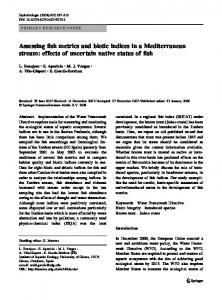
Table 3: Results of the MRE analysis for the data reported in Tab.2. in logistic regression), for other validation techniques. Another approach for assessing the predictive power of an eort estimation model is the Mean Magnitude of Relative Error (MMRE ), where MRE = 100 j(Real Effort , Estimated Effort)=Real Effortj. In Tab.3, the MMRE for data of Tab.2 are reported together with the Median Magnitude of Relative Error (MdMRE ), the Standard Deviation of MRE SDMRE , minimum and maximum MRE: MAXMRE and MINMRE respectively. The regression model adopted is tied to the residual analysis, and in particular to the assumption about the distribution of residuals. The residuals should be distributed as an independent normal random variable with zero mean and identical variance. In Fig.3 the residual distribution compared against a Normal(0,1) is reported. The shape shows how the two distributions are close each other. The distribution of residuals can be considered normal also because it has a mean value equal to 0; the skewness is 0.255 (a commonly used thumb-rule asserts that the distribution is normal if the skewness is in interval (-0.5, 0.5)); and kurtosis is close to 11 (with respect to 3 of a perfect normal) that shows a short-tail distribution. From this analysis, a normal distribution for residual can be assumed. Con rming the validity of the multilinear regression performed.

4.4 Metric Tuning Once the metrics are validated, they can be used for assessing projects for the speci c measuring context in which the weights have been evaluated. The same metric can be used in dierent Measuring Contexts with dierent weights for similar or dierent purposes. Moreover, as usually occurs, the measuring context usually changes with time { for example, until 1996, ELEXA factory produced controllers for low-price machines, now they are moving to produce high performance machines (project ICOOMM). Thus, metrics have been continuously revalidated in order to adjust the weights for tracking the evolution of a set of products. For instance, once a project maintained under control with CC metrics has reached its completion, predicted values can be compared with collected data. Causes of dierences have to be carefully analyzed. In general, if 0

17

0,5

Residuals Normal(0,1)

0,45 0,4

)UHTXHQF\

0,35 0,3 0,25 0,2 0,15 0,1 0,05

15

13

11

9

7

5

3

1

-1

-3

-5

-7

-9

-1 1

-1 3

-1 5

-1 7

0 -0,05

5HVLGXDOV

Figure 3: Residuals distribution compared with a Normal(0,1). project results are satisfactory, the collected data can be included into the values used for evaluating the general weights for the given measuring context. Otherwise, corresponding corrective actions have to be introduced. The set of values used for evaluating the weights must be carefully analyzed in order to correctly tune the model. For instance, the analysis of outliers and the analysis of dependencies of the metric terms can be used. In Fig.4, the dot diagram showing the scattering between eort and class complexity is reported. In this graph, the outliers are points located out of the bound lines marking the con dent limits [Rousseeuw et al. 1987]. The study of the outliers (values marked with letters) has to be associated with a deep analysis of the reasons for which those classes are far from the ideal correlation line [Rousseeuw et al. 1987], [Barnett et al. 1985]. This could be discussed together with the metric histograms. Outliers detection in single univariate sample can be easily identi ed, in a rst approximation, because they are very dierent from the others values of the sample. For more structured data, and especially for regression models the concept of outlier should be modi ed because it is not simply an extreme value, but it has a more general pattern-disrupting form. The outlier in multilinear regression models can impact largely on the model chosen for explaining data. This fact leads to take into account outliers and robust techniques for their estimation and accommodation [Barnett et al. 1985].

4.5 Thresholds and Reference Values In order to detect the presence of system dysfunctions, the adoption of reference values is quite frequent for discriminating when a metric value describes a problem on system/component. Frequently, systems/components are considered correct if the estimated metric value belongs to the range de ned within the maximum and minimum values. In some case the typical value is also given. For example, a too high NM may mean that the class is too large and, thus, very expensive to be maintained; a too high DIT means that the system presents a deep specialization hierarchy and, thus, it is becoming too complex to be reused. The relationship between the metric and feature has to be proven via a 18

250 x

200

estimated Effort

[ ]E 150

[ ]D

100 ( )B

( )C [ ]G

50

[ ]F ( )A [ ]H

0 0

50

100

150

200

250

observed Effort

Figure 4: Scattering diagram for CC (estimated eort) against observed eort (project LIOO). validation phase. The reference values used for detecting problems are typically set on the basis of the experience in several validation processes. In TAC++, their estimation can be performed on the basis of a statistical analysis of the reference projects and by considering the experience on past products. Thus, maximum and minimum values are evaluated for each speci c measuring context. The adoption of reference values is surely very useful for a fast detection of degenerative conditions. This approach is too simple when it is used on system level metrics. For example, assertions like \if the mean value of NM for the whole system is lower than a prede ned threshold, the costs of system maintenance will be acceptable" have to be carefully accepted. Thus, getting an out-of-bounds for a speci c metric for a certain class does not mean that the class has to be surely revised. Before correcting a problem, we have to be sure to have it. To this end, the results of a set of independent metrics have to be compared before deciding the intervention on a class. For example, a class can be very complex, but if it is reusable, veri able, testable, well-documented, etc., it is better to solve other problems rst, if any.

5 TAC++: Results Visualization and Interpretation In order to provide a fast and understandable view of the project status, the values obtained for LLMs and HLMs at system, class and method levels have to be visualized in a set of speci c views, pro les and histograms. Fig.5 depicts the relationships among the main components of TAC++ tool to manage these aspects: View Manager, Pro le Manager, Histogram Manager and Assessment Assistant. In the following subsections, the features of these components are described in detail. The views, pro les and histograms 19

are de ned and saved according to the measuring contexts for which they have been de ned. These graphs can be based on the LLMs, HLMs and data collected by the Collector. For this purpose, speci c graphic managers have been built. During the presentation of TAC++ components, guidelines to work with interpretation tools about the adoption of thresholds, reference values, diagram selection, application and interpretation for detecting problems from the assessment results are reported. These guidelines help the users to navigate on the large amount of information managed during the assessment.

Figure 5: TAC++: visualization of results and the Assessment Assistant. Dierent members of the development team may use TAC++ for dierent purposes. During the development life-cycle the system manager (project manager or control manager) has also the due to analyze the results produced by evaluating selected metrics and by comparing them with the corresponding company suggested bounds (by means of pro les). The results produced and their related actions for correcting any dierences with respect to the milestones planned (described in terms of the same indicators) are normally included in the project documentation. Typical actions for correcting 20

the values of the most important indicators should also be de ned in advance. For each measuring context and for each view, pro le and histogram, speci c textual comments should be added and shown to the user when reference values, pro les and distribution are exceeded. These have also to be collected in a development and management manual of the company. Even these comments need to be maintained and tuned according to the company evolution. The Histogram Manager can also draw normalized graphs (see Fig.5) with superimposed statistic curves in order to easily check if the system under assessment is suitable with respect to the Quality Manual speci cations of the company. Typical distributions of histograms can be assumed as reference patterns by the company. A collection of histograms among the various phases of the development life-cycle could aid the system manager to take into account the modi cations, from the point of view of quality pro le, of each class in the system. The Assessment Assistant provides support for system assessment by means of algorithms that reduce the complexity for inspecting the results and, thus, for detecting dysfunctions, and/or performing in automatic manner some processes.

5.1 Views and Pro les Graphic diagrams, typically called views and pro les, are needed for showing the assessment results with respect to typical and/or limit values. Two distinct de nitions are given for views and pro les. A collection of dierent metrics representing the same or related system/class features can be used and visualized in a single view with respect to bounds and typical values. Views are used to have an immediate and robust gure of system features { e.g., quality, eort for maintenance, eort for reuse, eort per subsystem, eort per work-package. The views can be employed for monitoring aspects of the system during its evolution, at methods, classes, and/or system levels. This is performed on the basis of the Life-Cycle Context for which they are de ned. In the views, the bounds (minimum and maximum acceptable values) can be considered as the limits out of which a further analysis (and may be a correction) should be needed. In a dierent visualization, minimum and maximum values can be those obtained from the whole system under analysis. In this way, it is quite clear how the class/subsystem under assessment is referred to the whole system. In any case, normalized graphs are used: Kiviat, star, pie, etc. In Fig.6, four Kiviat diagrams corresponding to four classes of LIOO project are reported. In this case, the maximum values (external circles) are evaluated on the whole system, while the dashed lines report the acceptable values estimated during the validation and imposed on the basis of the experience. In Fig.6, the views reported are related to classes marked as outliers in the scattering diagram of Fig.4. From these gures, it can be noted that most of the class features are out of the typical bounds and that the picture in lower-right corner has, for CI , NMI , CMICI , and NAI , values close to the maximum of the whole system. These metrics assert that the class inherits too much. In order to unify the actions to be performed for solving problems and for accelering their understanding, brief comments describing what should be done in the case of out-of-bounds, have to be de ned. In order to monitor class quality in project LIOO we de ned a view reporting values of metrics: NA, NM , CCm, CCGI and NSUP . Other typical examples of views are: (i) a view on class eort 21

Figure 6: Views (Kiviat's Diagrams) of some of the outliers identi ed in the previous scatter diagram (project LIOO). prediction: Size2, NAM and CC ; (ii) a view on class eort estimation: CCm , CCm , WMC , CL, CI , NAM and NAML; (iii) a view on eort prediction or estimation at system level: SC , TLOC , NCL, NRC and mean DIT ; (iv) a view on conformity to OOP at system level: NRC , NRC=NCL, SCm=NCL, Max(CC ) and Max(NAM ); (v) a view on class metrics related to re-usability and maintainability: NOC , NSUP , NSUB , DIT and NAI ; (vi) a view on class reusability: cognitive complexity, NAM , V I (Veri ability index) and CCGI . Typical actions to be performed when these metrics are out of the prede ned bounds are discussed in [Fioravanti et al. 1998b], [Fioravanti et al. 1998a], [Bucci et al. 1998]. The number of these diagrams for the whole system may become huge and, thus, their analysis fairly complex up to infeasible. For this reason, algorithms for navigating in the results produced by the assessment are needed (see Subsection 5.3). A pro le is a diagram in which the estimations of the several direct and indirect metrics are compared against expected values (reference value). For example, the quality pro le de ned on the basis of the 0

0

22

six features of the ISO 9126. In Fig.7, the expected pro les are compared with the estimated pro les in a normalized scale. Pro les are typically shown by using bars or Kiviat diagrams. Pro les can be used in any instant in which planned/reference measures can be compared against the actual values (see Fig.7 on the right, in which the eort planned for each system task is compared with respect to the actual eort). Another very important pro le is the Product Pro le. It includes: material costs for each piece, general costs, market level, potential reusability, etc. The structure of pro les (the number and selection of aspects to be controlled) is typically xed for all products of the factory/unit, while the speci c reference values may change for each product, e.g. to get a customized pro le.

Ar ch ite

ctu re Us D riv er er Us Iterf. er Su Ite p. rf. C MT onf. Co n Sim fig ula Er ror t +A or lar ms Do H cu me elp nta tio n

14 12 10 8 Prediction Estimation 6 4 2 0

Figure 7: On the left: project pro le according to the ISO 9126 quality standard. On the right: project pro le regarding predicted and estimated eort for tasks in men/month; evaluation performed close to the end of the development phase (project ICOOMM). In TAC++, both views and pro les can be de ned at method, class and system levels. The structure of views and pro les with their reference values can be organized according to the measuring context. Thus, actions and suggestions for solving problems in the case of detection of critical conditions can be customized for each speci c case. Dierent views can be de ned according to the needs of developers, subsystem managers and project manager [Nesi 1998].

5.2 Histograms At system/subsystem level, metrics can be used to analyze general system features (e.g., number of classes NCL, number of subsystems, number of root classes NRC , system complexity SC ) or as generic system component behavior (e.g., mean CC , mean NA, mean NM and mean NCL for subsystem). In this second case, the views are unsuitable for detecting troubles since the mean values can be within the correct bounds, but the system may present several out-of-bounds at class level. For this reason, it is important to analyze the distribution of each metric for the system under assessment. For example, by using histograms: (i) the number of classes for the complexity of classes, (ii) the number of methods for the complexity of methods, (iii) the number of classes for their CCGI , (iv) the number of classes for their NSUP , (v) the number of classes for their NSUB , etc. In Fig.8, the histogram of CCGI for project LIOO is reported. It is typically recommended, for reuse and understandability, to have classes with a CCGI close to 0.6. This allows the developers to use the class as a \black-box". For instance, in the example, by observing CCGI histogram, it is 23

evident that the peak is close to the suggested value. Some classes with a too low metric value are present; these classes are not observable enough and, thus, are expensive to be maintained and reused. It is suggested to check these classes in order to verify if the high internal complexity can be justi ed by their role in the system. In any case, the splitting of these large classes in more classes by using the well-known mechanism of delegation should be a good solution. It is also possible to identify classes for which the functional complexity is too high with respect to the interface complexity (CCGI close to 0). Owing to the tool used for collecting data, classes having CC = 0 have also been collected in this group and, thus, all classes de ned, but not yet implemented. Classes with CCGI = 1 are structures (according to C++) or have attributes and the external interface de ned, but the methods are not yet implemented. 35 ’CCGI1’ 30

Number Of Classes

25

20

15

10

5

0 -1

-0.5

0 0.5 1 Metric CCGI (early phase of development )

1.5

2

Figure 8: Histogram for CCGI , obtained at the rst checkpoint (project LIOO, version 0). Histograms are strongly useful since the adoption of bounds for detecting problems may lead to make large errors. In fact, according to the life-cycle context some out-of-bounds for some metrics and non well-behaved histograms (sensibly out of the reference distribution) may be accepted. For example, during the early development phase, the presence of de ned but not yet implemented classes has to be accepted without considering them as wrongly implemented classes. In fact, in the early phases the number of special cases can be too high to be manually managed. This problem frequently leads the assessment personnel to wait for a quite complete version before starting with the system assessment. Speci c metrics and tools may guide the assessment personnel in these phases. The result obtained by the scatter diagrams can be better analyzed if compared with the histogram of the corresponding metric. In Fig.9, the histogram of metric CC (estimated eort), related to the diagram of Fig.4 is shown. If the reference distribution is a Log Normal curve (as will be shown in Section 5.3), only some of the classes that are outliers in the scatter diagram are also out of the typical distribution histogram. In particular, classes: H, D and E should be more carefully inspected in order to verify the reasons of the dysfunction and to de ne action (if needed) to correct their behavior. Please note that the other classes have not been considered as aected by problems since they are within the reference histogram distribution. This means that in a system may exist few very complex classes. 24

These are typically called key and/or engine classes { [Lorenz et al. 1994], [Nesi 1998]. 8

7

Number of Classes

6

5

4

3

2

1

0 0

50

100

150

200

250

Metric CC

Figure 9: Histogram of metric CC as the estimated eort, related to the scatter diagram of Fig.4, (project LIOO). Histograms are a powerful tool for system assessment. In order to make histograms comparable with other systems and with reference distributions they have to be normalized. The typical distributions of the histograms for each metric have been extracted on the basis of the projects reported in the Introduction. Some typical distributions can be modeled as Gaussian, Log Normal curves. Normalized histogram distributions are quite independent of the development context, while are depending on the life-cycle context. In most cases, normalized histogram distributions are also independent of the languages { [Fioravanti et al. 1998a], [Lorenz et al. 1994]. Please note that the above-mentioned views, pro les and histograms are capable of analyzing the system aspects in a given time instant, in a given life-cycle context. In several cases, the single snapshot of the system status may produce insigni cant gures. This is more critical for metrics that are very sensitive to the development life-cycle phase. The trend analysis can be performed on metrics involved in views, pro les and histograms, and is speci cally needed to verify if the evolution of metrics is reaching the expected results. In some cases, the trend analysis can be performed for predicting future values by using some extrapolation algorithm, e.g., for predicting the cost of designing and coding in the phase of analysis [Fioravanti et al. 1999a].

5.3 Analysis of Assessment results The process of system assessment may produce a huge amount of data, typically analyzed by inspecting pro les, views, and histograms. A manual exhaustive analysis of graphs and diagrams is a very heavy, tedious and time consuming process. Moreover, the number of detected interventions per analyzed graph is really low. This is due to the fact that typically the largest part of the problems is relegated in a small system/subsystem part. For these reasons, and for the repetitive operations that have to be performed, the probability of producing errors in identifying real problems and thus on taking decisions 25

is quite high. In TAC++, according to the discussions performed in the previous sections, the elements manipulated during the assessment can be de ned as:

 Class 2 SubSystem, SubSystem 2 System, Class 2 System The system can be regarded as a set of subsystems and these in turn are sets of classes. Thus, generally, classes belong to the system, without loss of generality.

 Metrics These are used into views, pro les, and histograms with the associated reference bounds/distributions and weights (if any) on the basis of the measuring context and considering the feature that is intended to be estimated. Metrics formally hold only their de nition since the same metric can be used for dierent purposes with dierent weights.

 Profile  fmetric $ (feature; reference value; weights)g A Pro le is a collection of metrics related to features of class, subsystems or systems depending on its goals and on the measuring context (with reference value and weights). A pro le reports the speci c detailed features that have to be measured and their expected values along the software life-cycle. Pro les are more concise than views (pro les have only a reference value), thus they are more used at system or subsystem level.

 V iew  fmetric $ (feature; reference bounds; weights)g; fview suggestionsg A View is a collection of metrics related to features of classes, subsystems or systems depending on the view goals and on the measuring context. Reference bounds and weights depend on the measuring context and include minimum, maximum and typical values. A view identi es the speci c detailed features that have to be measured and their expected values along the software life-cycle. The views are a more general and powerful working tool than pro les and thus can be used in their place without restriction, but not the vice versa. For each view, a set of suggestions can be associated with the presence of out-of-bounds on a set of its metrics. These suggestions can be modi ed by the end-users. The suggestions cannot be associated with metrics since their meaning is context dependent and may depend on more than one metric.

 Histogram  metric $ (reference distribution; weights); fhistogram suggestionsg A Histogram reports the distribution of the metric behavior on the whole system/subsystem. For each histogram, a set of suggestions can be associated with the presence of out-of-distribution. These suggestions can be changed by the end-users. The suggestions cannot be associated with metrics since their meaning is context dependent. For system level assessment, speci c pro les are typically de ned for annualizing eort, quality, etc. The collection of features analyzed via metrics depends on these pro le goals. These are typically mean values of class metrics (mean CC , mean NAM , mean NAML, mean CCGI , etc.) or structural 26

consumptive metrics (NRC , NCL, SC , etc.). In the assessment phase, the estimated values are compared with the reference values (the reference pro le). The detection of a problem (a relevant dierence between expected and estimated value) by means of a system level metric may be considered as an alarm for the system life-cycle process. Once detected at system level, the same or a corresponding problem may be found into one or more subsystems. On the other hand, the lack of detectable problems in the system (subsystem) pro le/view may make the general manager satis ed but does not guarantee the lack of problems in the subsystems (classes). This fact constraints subsystem managers and quality control personnel to analyze all system classes with speci c views in systematic manner to look for problems. At system level, the presence of out-of-bounds can be identi ed by de ning speci c consumptive metrics for reporting problems at systems (subsystem). These can be based on the results produced at lower level, subsystem (class). This can be obtained by de ning metrics such as: maximum value of CC among the system (subsystem) classes, maximum value of NAML among the system (subsystem) classes, etc. This kind of consumptive metrics are useful for the fast automatic detection of out-ofbounds; on the other hand, they are too simple since the presence of out-of-bounds does not always imply the needs of intervention; thus a further inspection at class level is consequently needed. On the other hand, metrics based on the mean value of class level metrics are totally unuseful since a correct mean value may hide a lot of undesirable instances of unsatisfactory values. In the following, an algorithm for partially automating the assessment process is proposed. It has been de ned for automatically combining results coming from views and histograms. This reduces the number of views that have to be analyzed during the assessment. The algorithm has been implemented into the so-called Assessment Assistant inside the TAC++ tool.

5.3.1 Assessment Assistant Algorithm Once de ned the views with their metrics on the basis of the experience and by using the results of validation phases, the set of views and related histograms can be used for system assessment in a systematic manner. For example, if the assessment of a (sub)system is based on 4 views with 6 metrics each, and it has 1000 classes, then the tool for system assessment has to estimate 24000 metric values. Their estimation is not a problem with the support of suitable automatic tools, but a real-time estimation is frequently needed for small projects or subsystems. The main problem is that system classes have to be analyzed by specialized personnel via 4000 Views, 4 views per class. The computational complexity of an exhaustive analysis by means of views is an O(C V M ) (considering the comparison with the reference value as the dominant operation); where: C is the number of classes per (sub)system, V the number of views per class, M the mean number of metrics involved in each view. Please note that a metric can be used in dierent views for dierent purposes, with dierent bounds. Thus, in these conditions, the complexity of the assessment process is too heavy to be performed in short time and without errors. A partial screening of the 4000 views can be performed by considering as classes that need of a further analysis only those having more than  metrics out of the suggested bounds (for instance, with the number of out-of-bounds bigger than a value, ). The value of  can be tuned 27

according to the goals used. In order to make easier and faster the assessment process, an algorithm has been de ned and implemented. The main idea behind the algorithm is the adoption of the histogram as the main vehicle for detecting problematic classes. According to the above numerical example, the histograms to be analyzed are only 24. In order to make histograms of a (sub)system comparable with those of other (sub)systems and with the reference distributions they have to be normalized (see Fig.10). The normalization has to be performed on both axes on the basis of the total number of classes. To this end, in the histogram: (i) X-axis is divided in a number of categories for collecting classes having similar metric value and ranges from 0 to the maximum of the metric in the (sub)system or to the maximum number of categories; (ii) Y-axis ranges from 0 to 1, from 0 classes per category to 1 when all classes belong to the same category. It is possible to pass from the category to the metric value by using the scale factor, F . In Fig.10, each graph presents the histograms of the same system in two dierent phases. The project LIOO has been totally reused into project MOODS and thus has changed name. Observing the graphs, the evolution of the histogram distributions is clear. The typical distributions of the histograms for each metric have to be extracted on the basis of reference projects and can be modeled as Gaussian, Log Normal curves, etc. depending on the metric. The reference distribution de nes the percentage (and thus the number) of classes that may belong to a certain category. This may present the metric value in a certain range. Normalized histograms may present several classes out of the histogram distribution in the correspondence of their mean value or close to the zero. These classes may be considered correct depending on the metrics used. In order to verify if the sample data for each distribution can be generated from a standard distribution like a Normal or LogNormal, the Kolmogorov-Smirnov One Sample Statistic has been adopted. For this test the null hypothesis, H0, consists in assessing that the samples can be drawn from a prede ned distribution, while the alternative hypothesis, H1, asserts that it is not possible to draw the samples from the chosen distribution. In particular, the signi cance level for rejecting the null hypothesis has been imposed to 0.05. Under this condition for a number of samples equal to 116 (LIOO, version 3) the critical Distance for rejecting H0 is D=0.124, while for a number of samples equal to 186 (MOODS, version 1) is D=0.098. Values lower or equal than those reported con rm that data can be considered as belonging to the supposed distribution. In Tab.4, the values related to the validation of the typical histogram distributions are reported. With the same technique, it has been demonstrated that histogram distributions depend on the development and life-cycle context as shown in Tab.4 where the results of the Kolmogorov-Smirnov test on the distributions of LIOO (version 3) and MOODS (version 1) have been reported. For the test, the H0 hypothesis states that the two samples are drawn from the same distribution; then, H1 states that the distributions are dierent. H0 has been rejected, and then the distribution are dierent (D = 0:37 and p-val=0.0000). This is mainly due to the dierent mean values that distributions provide. According to the histogram distribution, some classes are considered correct even if they present values typically out of the imposed bounds for the metric. This is due to the fact that histograms evaluate the distribution of the metric value in the system and, thus, classes under the rst part of distribution tails are considered as belonging to the general system behavior and not aected by 28

0.5 0.45

&&*,

LIOO3 MOODS1 Normale

0.4

&&

0.45

LIOO3 MOODS1 LogNormal

0.4

0.35 0.35 0.3 0.3 0.25 0.25 0.2 0.2 0.15 0.15 0.1 0.1 0.05 0.05 0 0

0.1

0.2

0.3

0.4

0.5

0.6

0.7

0.8

0.9

0.999999

1 0 1

-0.05

2

3

4

5

6

7

8

9

10

11

12

13

14

15

16

17

18

19

20

21

22

23

24

25

26

0.4

0.4

1683

LIOO3 MOODS1 LogNorm

0.35

LIOO3 MOODS1 LogNorm

1$0

0.35

0.3

0.3

0.25 0.25

0.2 0.2

0.15 0.15

0.1 0.1

0.05 0.05

0 0

10

20

30

40

50

60

70

80

90

100 110 120 130 140 150 160 170 180 190 200 210 220 230 240

0 0

1

2

3

4

5

6

7

8

9

10

-0.05

0.6

0.6

LIOO3

LIOO3

&/

&,

MOODS1

MOODS1 LogNorm

LogNorm

0.5

0.5

0.4

0.4

0.3

0.3

0.2

0.2

0.1

0.1

0

0 1

3

5

7

9

11

13

15

17

19

21

23

25

27

29

31

33

35

37

39

41

43

45

1 2

47

3

4 5

6

7 8

9 10 11 12 13 14 15 16 17 18 19 20 21 22 23 24 25 26 27 28 29 30 31 32 33 34 35 36 37 38 39 40 41

Figure 10: Each histogram contains the distribution estimated for project MOODS (version 1) and LIOO (version 3) and the reference distribution for the context of LIOO, version 3. Please consider scale factors F reported on Tab.6 for estimating the metric values.

problems. On the other hand, the adoption of simple bounds on the metric value marks these classes as aected by problems. According to our experience, both the approaches can be used. The combination of both the techniques is a more robust approach to identify classes that surely need an intervention. The algorithm reported in Fig.11 has been de ned and implemented in TAC++ for processing the results of the assessment in order to identify in automatic manner the classes that have relevant problems. As already stated, we consider as relevant problems those which lead classes to be out-ofbound in the view and out-of-distribution in the corresponding histogram. This means that the class metric presents unacceptable value and that in the distribution the class belongs to a category out of typical histogram distribution. The system is analyzed on the basis of the measuring context (context plus phase plus level in the algorithm). On this basis, a set of Views are identi ed (as above de ned) with their corresponding 29

Metric CCGI CCGI NAM

Distribution Type Normal Normal LogNormal

project version Mean-Value Std. Dev. distance D p-value LIOO 3 0.59 0.15 0.1030 0.161 MOODS 1 0.63 0.21 0.0936 0.072 LIOO 3 1.59 0.45 0.1218 0.059

Table 4: Data of metric distributions validated with Kolmogorov-Smirnov statistic test. The values of mean and standard deviation are those that allow obtaining a p-value for the corresponding project for demonstrating that the distribution can model the data. metrics and reference values. From these Views all the related Metrics are extracted. In a rst phase, the histograms of these metrics are automatically inspected in order to exact the classes which are out of the reference distribution, ClassesOutOfDistrib[m], for each metric, m, in at least a histogram. To work only with out-of-distribution classes is a relevant reduction with respect to the analysis of all classes. The extraction of out-of-distribution classes, with ExtractClasses(), has to be based on the knowledge of a reference distribution for the histogram, and is performed by extracting classes that belong to categories in which the number of classes is too high with respect to the planned value of the reference histogram distribution. In the second phase, each class of the union of all ClassesOutOfDistrib[i] is analyzed to verify if it provides out-of-bounds in the views and if these are also out-of-distribution. To this end, for each view the metrics out-of-bounds, MetricsOutOfBounds, are extracted. Then, for each class metric it is veri ed if the class is also out-of-distribution. With this process, for each class and view the set of CriticalMetrics which are both out-of-bounds and out-of-distribution are extracted. Finally, if the number of critical metrics in the view is bigger than  the algorithm considers the class as aected by a problem and thus suggested actions are searched in both the related view and histogram repositories. The user can customize the corrective actions. Suggested by the Assessment Assistant and the related rules for their presentation. The second phase of the algorithm has a computational complexity which is an O(KOD V M ); where KOD is the number of classes which have at least an out of histogram distribution. The global complexity of the algorithm is lower than the complexity obtained for the systematic analysis based on classes. It is an O(C V M ); since typically, KOD  C . The algorithm takes advantage from the reduction of the number of classes to be analyzed and avoids the inspection of all views for each class. The methodology and algorithm have been used in several assessment phases in the projects mentioned in the introduction. After a validation phase, the algorithm has been also implemented in the Assistant Assessment of TAC++ tool. In the next subsection, an example of the adoption of the Assistant Assessment for a real project is reported.

5.3.2 Working with the Assistant Assessment The following example is mainly referred to project LIOO version 3. In this case, 4 views have been used. The rst view includes metrics related to: development eort (CC , CL, CI and NAM ), hierarchy (NSUP ) and comprehensibility (CCGI ); eort prediction or estimation at system level: SC , TLOC , 30

8 SubSystem 2 System

begin

level = SubSystem:AnalysingLevel(Who); context = SubSystem:DevelopmentContext(level); phase = SubSystem:LifeCyclePhase(level; context); V iews = V iewRepositor:Select(level; context; phase); Metrics = Metrics:Extract(V iews); 8 i 2 Metrics ClassesOutOfDistrib[i] = ;; 8 m 2 Metrics

begin

histogram = SubSystem:Histogram(m); ClassesOutOfDistrib[m] = ClassesOutOfDistrib[m] [ histogram:ExtractClasses(level; context; phase);

endbegin

S 8 class 2 Metrics ClassesOutOfDistrib[i] i

begin 8 view 2 V iews begin

CriticalMetrics = ;; MetricsOutOfBound = view:Check(class); 8 metric 2 MetricsOutOfBound

begin if class 2 ClassesOutOfDistrib[metric] then CriticalMetrics = CriticalMetrics [ metric; endif endbegin if NumberOf(CriticalMetrics) >  then

ActionSuggested = view:CorrectiveAction(CriticalMetrics);

8 metric 2 CriticalMetrics

begin

histogram = metric:getHistogram(level; context; phase); ActionSuggested = ActionSuggested [ histogram:CorrectiveAction(metric);

endbegin endif endbegin endbegin endbegin

InteractiveV isualization(class; ActionSuggested);

Figure 11: Assistant Assessment algorithm for automating the result screening and understanding.

NCL, NRC and mean DIT ; conformity to OOP at system level: NRC , NRC=NCL, SCm=NCL, Max(CC ) and Max(NAM ); re-usability and maintainability: NOC , NSUP , NSUB, DIT and NAI ; for a total of 21 dierent metrics in the 4 views. The following data has been obtained by using the above-presented algorithm for system assessment. The example has a relevance only for showing the evolution of the number of classes identi ed as needing intervention and not for the speci c values used for the metrics. These may have a relevance only for the speci c measuring context used. In Tab.5, the number of classes that have been detected out-of-bounds for each metric in project LIOO (version 3), KOB , are reported. The reference bounds used in the above-mentioned rst view for identifying classes that may need a further inspection are reported: minimum and maximum values. The bounds depend on the measuring context. In this case, the project was assessed in the rst part 31

of its development life-cycle. The bounds are typically very strict (close to the typical mean values) with respect to the bound values which are used for the same metrics in the case of the class selection only via out-of-bounds (see the second part of the table). Please note that when large bound values (distant from the typical mean value) are used, a lower number of classes are selected. Large bounds are typically used for reducing the number of classes to be inspected. Moreover, the bounds have to be substituted with strict bounds when the algorithm is used to identify classes with problems by using both bounds and distributions. strict bounds, project LIOO ver.3 Metric minimum maximum KOB CCGI 0.5 0.70 49 CC 0.0 600.0 32 NSUP 0.0 4 1 NAM 0.0 50 31 CL 0.0 400.0 8 CI 0.0 600.0 9

large bounds, project LIOO ver.3 Metric minimum maximum KOB CCGI 0.5 1 31 CC 0.0 1500.0 16 NSUP 0.0 5 0 NAM 0.0 90 21 CL 0.0 700.0 5 CI 0.0 1200.0 1

Table 5: Number of identi ed out-of-bounds classes per metric ( rst view) for project LIOO (ver. 3) and related bounds: above the bounds corresponding to correct measuring context; below the large bound values which are typically used in simple approaches based only on out-of-bounds. In Tab.6, the data of the reference histogram distributions for the metrics related to a view used in the example are reported. Each reference histogram distribution is de ned on the basis of its basic curve (Hist.Distribution in the table), mean value, standard deviation, and the scale factor, F . In this context, F can be used for interpreting the graphs reported in Fig.10. The correlations have been estimated by considering the distribution of metric values in the system and the reference distributions reported in Tab.6. The table reports also the number of classes that have been detected to be out of the reference distribution for each histogram (metric in the view) in project LIOO version 3, KOD . Metric

CCGI CC NSUP NAM CL CI

histogram distributions parameters, Project LIOO ver.3 Hist.Distribution mean value Std. Dev. F KOD Correlation With Distribution Norm 0.6 0.1 1 64 0.86 LogNorm 1.0 0.3 100 32 0.84 LogNorm 1.0 0.45 1 0 0.86 LogNorm 1.4 0.4 10 28 0.79 LogNorm 0.6 0.8 20 18 0.81 LogNorm 1.0 0.5 50 28 0.85

Table 6: Number of identi ed out-of-distribution classes for the metrics related to the rst view for project LIOO (version 3); and related mean values and standard deviations. Typically, classes presenting 1 or more out-of-bounds or out-of-distributions in the selected view metrics are considered as problematic and thus they need a further inspection. This approach, in most cases, produces a too high number of classes that have to be inspected. In order to reduce this high number of classes (thus, the eort for their analysis) the metric bounds are typically enlarged (see Tab.5). On the other hand, in this manner, classes with problems (that need to be furtherly inspected) risk to 32

pass the selection without any problem, leaving the system to grow towards degenerative conditions. By using the above-presented algorithm, this problem is strongly reduced. This has been veri ed by observing the eects of dierent criteria for selecting critical classes, as reported below against the results produced by an exhaustive analysis. The Number of Selected Classes, NSC , to be inspected and revised can be estimated on the basis of dierent criteria, that are the Detection Metrics: NCL X NSC (DMi) = gc(DMi; ); c

where: gc (DMi ; ) is a function of the generic detection metric, DMi , and threshold , on a view of class c:  gc(DMi; ) = 10 ifelseDMi >  : DMi can be a detection metric considering the Out-of-Bounds, OB , or the Out-of-Distributions, OD. Dierent Detection Metrics have been de ned as reported in Tab.7, where: OBm states if metric m is out-of-bound or not, ODm states if metric m is out-of-distribution or not, and function istrue() return a value equal to 1 if its parameter is out. In Tab.7, the following detection metrics have been de ned: DMOB for counting the number of metrics of out-of-bounds in a class view; DMOD for counting the number of metrics of out-of-distribution in a class view; DM for counting the number of metrics which are out-of-bounds and out-of-distribution for the same class view; DM for counting the number of metrics which are out-of-bounds or out-of-distribution for a class view; DM+ for counting the number of metrics which are out-of-bounds plus those which are out-of-distribution for a class view. Therefore, with NSC () is possible to count critical conditions according to dierent detection criteria. ^

_

DM metricPde nition CC DMOB = Pm2V iew istrue(OBm ) out DMOD =P m2view istrue(ODm ) out DM^ = Pm2V iew istrue(OBm ^ ODm ) out DM_ = m2V iew istrue(OBm _ ODm ) out DM+ = DMOB + DMOD 2 out

View with 6 metrics

CL CI NAM NSUP CCGI value in out out in in in out out out out

out out out out 2 out

in in in in in

out in in out out

4 3 2 5 7

Table 7: De nition of Detection Metrics and a counting example for a View with 6 metrics, for m = 1::6: CC , CL, CI , NAM , NSUP , CCGI . In Tab.8, the data related to the application of detection metrics in the counting of NSC have been combined as a function of  for the rst view of LIOO project, version 3; where the percentage of saving for the generic Detection Metric, DMi , is estimated by using: +) , NSC (DMi) 100: percentage of saving (DMi) = NSC (DM NSC (DM+) When NSC (DM+) is used as the main criterion for detecting classes that need a further analysis, a larger number of classes are identi ed. If this approach for identifying classes with problems is performed on all views a very large percentage of classes are selected, in the above case we reached the 93%. This very high number of classes is obviously impossible to be managed and has no sense. This 33



0 1 2 3 4 5 6 7 8 9 10

NSC (DMOB ) NSC (DMOD ) NSC (DM^ ) NSC (DM_ ) NSC (DM+ ) % of saving (DM^) 53 34 26 14 2 1 0 0 0 0 0

79 50 25 11 5 0 0 0 0 0 0

45 29 15 11 1 0 0 0 0 0 0

87 54 28 23 6 1 0 0 0 0 0

87 59 40 31 26 24 14 11 6 1 1

48 51 62 64 96 100 100 100 100 100 100

Table 8: Number of selected classes, NSC (DMi), as a function of  for the rst view: project LIOO version 3 with 116 classes. eect is also present (even if in lower manner) when large bound values are used. The percentage of saving for the DM -based solution has been estimated with respect to DM+ -based solution since this is the typically used approach for selecting classes that need a further inspection. From the table, it is clear that it is possible to obtain a number of selected classes, NSC (DM+), comparable with that obtainable by using a dierent value of  or by using dierent values for bounds by NSC (DMOB ) or NSC (DMOD). On the other hand, these last detection metrics for identifying the critical classes are not equivalent, they share great part of the same classes but not all as it can be seen comparing NSC (DMOD) and NSC (DMOB). A dierent approach is to consider the operation of conjunction and disjunction for identifying the number of selected classes. For higher values of , a higher percentage of saving (in terms of classes to be analyzed) is obtained by using DM instead of DM+ . This distribution is also present when the percentage of saving is estimated with respect to either NSC (DMOB) or NSC (DMOD) or NSC (DMO). Therefore, the more restrictive detection metric is DM . In this case, an  = 3 was considered and thus 11 classes were analyzed. Among these, we discovered that only 3 classes were aected by real design problems. These classes were the same classes identi ed by quality control personnel by performing a manual exhaustive analysis of views. Only two of these classes were included in those identi ed by NSC (DMOB) or by NSC (DMOD) for  = 4. Similar results have been obtained for other projects mentioned in the introduction. For this reason, it is convenient to adopt an  equal 2 or 3, obtaining a time saving of about 40 % with respect to working only with bounds or distributions and about a 90 % with respect to the exhaustive analysis. ^

^

^

6 Conclusions The tool described in this paper has been developed during the last years during the assessment and control of several industrial and Academic projects. Some of these have been multipartner ESPRIT projects { e.g., ICCOC ESPRIT HPCN, MOODS ESPRIT HPCN, MUPAAC ESPRIT HPCN. During the last few year, a tool has been pro tably used for both metrics and system assessment. Together with 34

the tool we identi ed a collection of guidelines and suggestion that can be considered a sort of modus operandi to work with metrics in order to detect analysis and design problems, and for eort estimation and prediction. Operatively, the methodology provides a set of diagrams: views, pro les and histograms and the strategies for their adoption and the corresponding guidelines for their interpretation. The methodology and related visualization facilities are fully supported by TAC++ tool. In the paper, some suggestions to avoid confusion and time consuming in processing results and choosing metrics for views and pro les have been also given. The authors' experience in interpreting assessment results and de ning a methodology for product assessment along its life-cycle has been reported. By interpreting the suggested diagrams in the proposed manner a clear picture of the system under assessment can be obtained, and the detection of system dysfunction during the development life-cycle is possible and fast. The assistant assessment algorithm has been pro tably adopted reducing the detection and intervention time.

Acknowledgements

The authors would like to thank all the members of TAC++ team and the many other people involved in its development. Deep thanks also to the many people involved in the several projects managed by one of the authors. A special thank to B. Pages for an early version of the class browser. A particular thank to Prof. G. Bucci for his suggestions and encouragement.

References [Albrecht et al. 1983] [Barnett et al. 1985] [Basili et al. 1983a] [Basili et al. 1983b] [Basili et al. 1984] [Basili et al. 1994] [Basili et al. 1996]

A. J. Albrecht and J. E. GaneyJr. Software function, source lines of code, and development eort prediction: A software science validation. IEEE Transactions on Software Engineering, 9(6):639{648, Nov. 1983. V. Barnett and T. Price. Outliers in Statistical Data. John Wiley & Sons, USA, 1985. V. R. Basili and D. H. Hutchens. An empirical study of a syntactic complexity family. IEEE Transactions on Software Engineering, 9(6):664{672, Nov. 1983. V. R. Basili, R. W. SelbyJr, and T.-Y. Phillips. Metric analysis and data validation across fortran projects. IEEE Transactions on Software Engineering, 9(6):652{663, Nov. 1983. V. Basili and D. M. Weiss. A methodology for collecting valid software engineering data. IEEE Transactions on Software Engineering, 10(6):728{738, 1984. V. Basili, C. Caldiera, and H. D. Rombach. Goal question metric paradigm. Encyclopedia of Software Engineering (Marciniak, J.J., ed.), John Wiley & Sons, 1:528{532, 1994. V. R. Basili, L. Briand, and W. L. Melo. A validation of object oriented design metrics as quality indicators. IEEE Transactions on Software Engineering, pages 751{761, Oct 1996.

35

[Behrens 1983] [Bellini et al. 1999] [Booch 1996] [Briand et al. 1998a] [Briand et al. 1998b]

[Briand et al. 1998c] [Briand et al. 1999a] [Briand et al. 1999b] [BritoeAbreu et al. 1995] [Bucci et al. 1998] [Butera et al. 1998]

[Chidamber et al. 1994] [Chidamber et al. 1998] [Coulange et al. 1993]

C. A. Behrens. Measuring the productivity of computer systems development activities with function points. IEEE Transactions on Software Engineering, 9(6):648{652, Nov. 1983. P. Bellini, F. Fioravanti, and P. Nesi. Managing music in orchestras. IEEE Computer, pages 26{34, September 1999. G. Booch. Object Solutions, Managing the Object-Oriented Project. AddisonWesley, Menlo Park, California, USA, 1996. L. Briand, J. W. Daly, V. Porter, and J. Wurst. A comprehensive empirical validation of product measures for object oriented systems. Technical report, Technical Report ISERN-98-07, ISERN, Germany, 1998. L. Briand, J. Wurst, S. Ikonomovski, and H. Lounis. A comprehensive investigation of quality factors in object oriented designs: an industrial case study. Technical report, Technical Report ISERN-98-29, IESE-47988e, IESE, Germany, 1998. L. C. Briand, J. Wust, J. W. Daly, and D. V. Porter. Exploring the relationships between design measures and software quality in object oriented systems. Journal of Systems and Software, 1998. L. C. Briand, J. W. Daly, and J. K. Wust. A uni ed framework for coupling measurement in object oriented systems. IEEE Transactions on Software Engineering, 25(1):91{120, January/February 1999. L. C. Briand, J. Wust, and H. Lounis. Using coupling measurements for impact analysis in object oriented systems. In Proc. of the IEEE International Conference on Software Maintenance. IEEE Press, Sept. 1999. F. BritoeAbreu, M. Goulao, and R. Esteves. Toward the design quality evaluation of object oriented software systems. In Proc. of 5th International Conference on Software Quality, Austin, USA, Oct. 1995. McLean. G. Bucci, F. Fioravanti, P. Nesi, and S. Perlini. Metrics and tool for system assessment. In Proc. of the IEEE International Conference on Complex Computer Systems, pages 36{46, California, USA, August 1998. F. Butera, B. Fontanella, P. Nesi, and M. Perfetti. Reengineering a computerized numerical control towards object-oriented. In Proc. of the 2nd Euromicro Conference on Software Maintenance and Reengineering, Florence, Italy, 8-11 March 1998. IEEE Press. S. R. Chidamber and C. F. Kemerer. A metrics suite for object oriented design. IEEE Transactions on Software Engineering, 20(6):476{493, June 1994. S. R. Chidamber, D. P. Darcy, and C. F. Kemerer. Managerial use of metrics for object oriented software: An exploration analysis. IEEE Transactions on Software Engineering, 24(8):629{639, August 1998. B. Coulange and A. Roan. Object-oriented techniques at work: Facts and statistics. In Proc. of the International Conference on Technology of Object-Oriented

36

Languages and Systems, TOOLS Europe 93, pages 89{94, Versailles, France, 8-11

[Daly et al. 1995] [Dunteman 1989] [Fagan 1986] [Fioravanti et al. 1998a] [Fioravanti et al. 1998b]

[Fioravanti et al. 1999a]

[Fioravanti et al. 1999b] [Halstead 1977] [Henderson-Sellers 1991] [Henderson-Sellers 1993]

March 1993. J. Daly, J. Miller, A. Brooks, M. Roper, and M. Wood. Issues on the objectoriented paradigm: A questionnaire. Technical report, Dept. of Computer Science, Univ. of Strahclyde, UK, RR-95-183, June 1995. G. Dunteman. Principal Component Analysis. Sage University Paper, 07-69, Thousand Oaks, CA, USA, 1989. M. E. Fagan. Advances in software inspections. IEEE Transactions on Software Engineering, 12(7):744{751, July 1986. F. Fioravanti, P. Nesi, and S. Perlini. Assessment of system evolution through characterization. In Proc. of the IEEE International Conference on Software Engineering, pages 456{459, Kyoto, Japan, April 1998. F. Fioravanti, P. Nesi, and S. Perlini. A tool for process and product assessment of c++ applications. In Proc. of the 2nd Euromicro Conference on Software Maintenance and Reengineering, pages 89{95, Florence, Italy, 8-11 March 1998. IEEE Press. F. Fioravanti, P. Nesi, and F. Stortoni. Metrics for controlling eort during adaptive maintenance of object oriented systems. In Proc. of the IEEE International Conference on Software Maintenance, pages 483{492, Oxford, England, Sept. 1999. IEEE Press. F. Fioravanti, P. Nesi, and M. Polo Usaola. Complexity/size metrics for objectoriented systems. Technical report, University of Florence, TR 17/99, Florence, Italy, 1999. H. M. Halstead. Elements of Software Science. Elsevier North Holland, 1977. B. Henderson-Sellers. Some metrics for object-oriented software engineering. In Proc. of the International Conference on Technology of Object-Oriented Languages and Systems, TOOLS 6 Paci c 1991, pages 131{139. TOOLS USA, 1991. B. Henderson-Sellers. The economics of reusing library classes. Journal of Object Oriented Programming, pages 43{50, July-August 1993.

[Henderson-Sellers 1994]

B. Henderson-Sellers. Identifying internal and external characteristics of classes likely to be useful as structural complexity metrics. In D. Patel, Y. Sun, and S. Patel, editors, Proc. of International Conference on Object Oriented Information Systems, OOIS'94, pages 227{230, London, Dec. 19-21 1994. Springer Verlag. [Henderson-Sellers 1996] B. Henderson-Sellers. Object Oriented Metrics. Prentice Hall, New Jersey, 1996. [Henderson-Sellers et al. 1990] B. Henderson-Sellers and J. M. Edwards. The object oriented systems life cycle. Communications of the ACM, 33(9):143{159, Sept. 1990. [Henderson-Sellers et al. 1994] B. Henderson-Sellers, D. Tegarden, and D. Monarchi. Metrics and project management support for an object-oriented software development. In Tutorial Notes TM2, TOOLS Europe'94, International Conference on Technology of ObjectOriented Languages and Systems, Versailles, France, 7-10 March 1994.

37

[Henry et al. 1981] [HosmerJr et al. 1989] [Kemerer 1987] [Kemerer et al. 1999] [Laranjeira 1990] [Li et al. 1987] [Li et al. 1993] [Lorenz et al. 1994] [Low et al. 1990] [McCabe 1976] [Meyer 1990] [Nesi 1998] [Nesi et al. 1996] [Nesi et al. 1998] [Rousseeuw et al. 1987] [Schneidewind 1992] [Schneidewind 1994] [Shepperd et al. 1993]

S. Henry and D. Kafura. Software structure metrics based on information ow. IEEE Transactions on Software Engineering, 7(5):510{518, 1981. D. W. HosmerJr and S. Lemeshow. Applied Logistic Regression. Jhon Wiley & Sons, New York, USA, 1989. C. F. Kemerer. An empirical validation of software cost estimation models. Communications of the ACM, 30(5):416{429, May 1987. C. F. Kemerer and S. Slaughter. An empirical approach to studying software evolution. IEEE Transactions on Software Engineering, 25(4):493{509, July/Aug. 1999. L. A. Laranjeira. Software size estimation of object-oriented systems. IEEE Transactions on Software Engineering, 16(5):510{522, 1990. H. F. Li and W. K. Cheung. An empirical study of software metrics. IEEE Transactions on Software Engineering, 13(6):697{708, June 1987. W. Li and S. Henry. Object-oriented metrics that predict maintainability. The Journal of Systems Software, 23:111{122, 1993. M. Lorenz and J. Kidd. Object-Oriented Software Metrics, A Practical Guide. PTR Prentice Hall, New Jersey, 1994. G. C. Low and D. R. Jeery. Function points in the estimation and evaluation of software process. IEEE Transactions on Software Engineering, 16(1):64{71, Jan. 1990. T. J. McCabe. A complexity measure. IEEE Transactions on Software Engineering, 2(4):308{320, 1976. B. Meyer. Tools for the new culture: Lessons learned from the design of the eiel libraries. Communications of the ACM, 33(9):68{88, 1990. P. Nesi. Managing oo projects better. IEEE Software, pages 12{24, July-Aug 1998. P. Nesi and M. Campanai. Metric framework for object-oriented real-time systems speci cation languages. The Journal of Systems and Software, 34:43{65, 1996. P. Nesi and T. Querci. Eort estimation and prediction of object-oriented systems. The Journal of Systems and Software, Vol 42:89{102, 1998. P. J. Rousseeuw and A. M. Leroy. Robust Regression and Outlier Detection. Jhon Wiley & Sons, New York, USA, 1987. N. F. Schneidewind. Methodology for validating software metrics. IEEE Transactions on Software Engineering, 18(5):410{421, May 1992. N. F. Schneidewind. Validating metrics for ensuring space shuttle ight software quality. Computer, pages 50{57, August 1994. M. Shepperd and D. Ince. Derivation and Validation of Software Metrics. Clarendon Press, Oxford, 1993.

38

[Stetter 1984] [Thomas et al. 1989] [Zuse 1994] [Zuse 1998]

F. Stetter. A measure of program complexity. Computer Language, 9(3):203{210, 1984. D. Thomas and I. Jacobson. Managing object-oriented software engineering. In

Tutorial Note, TOOLS'89, International Conference on Technology of ObjectOriented Languages and Systems, page 52, Paris, France, 13-15 Nov. 1989. H. Zuse. Quality measurement { validation of software metrics. In Proc. of the 7th International Software Quality Week in San Francisco, QW'94, pages 4{T{2.

Software Research, 17-20 May 1994. H. Zuse. A Framework of Software Measurement. Walter de Cruyter, Berlin, New-York, 1998.

Paolo Nesi received the Laurea degree in Electronic Engineering from the University of Florence,

Italy, in 1987. He is currently Associate Professor at the University of Florence, Department of Systems and Informatics. Previously he was assistant professor at University of Florence and visiting researcher at the IBM Almaden Research Center, USA. He received his Ph.D. in computer engineering from University of Padoa. He has been Chair of several international conferences in the area of software engineering. He serves in the Program and organization committees of several international conferences, journals and book series. He holds the scienti c responsibility at CESVIT for HPCN (High Performance Computer and Networking). He has been responsible for several national and international multipartner research projects, in the area of software engineering. He has published more than 110 research papers on journals and conference proceedings. His research interests include: software assessments, metrics, formal languages, object-oriented, reengineering and maintenance.

Fabrizio Fioravanti took his Ph.D. in Software and Telecommunication Engineering at the Uni-

versity of Florence. He obtained the Laurea degree in Electronic Engineering from the same University in 1996. He is currently Assigned Professor on Computer Architecture at the University of Florence. He has been actively involved in the organization of international conferences.

39

Contents 1 Introduction

1

2 Overview of Object-Oriented Metrics

4

3 General Architecture of TAC++

9

2.1 Eort Estimation and Prediction Metrics . . . . . . . . . . . . . . . . . . . . . . . . . . 2.2 Metrics for Assessing System Structure and Quality . . . . . . . . . . . . . . . . . . . .

4 TAC++: Metric Estimation, Tuning and Validation 4.1 4.2 4.3 4.4 4.5

Low Level Metrics and Data Collector . . High Level Metrics . . . . . . . . . . . . . Metric Validation and Measuring Context Metric Tuning . . . . . . . . . . . . . . . . Thresholds and Reference Values . . . . .

. . . . .

. . . . .

. . . . .

. . . . .

. . . . .

. . . . .

5 TAC++: Results Visualization and Interpretation 5.1 Views and Pro les . . . . . . . . . . . . . . . . 5.2 Histograms . . . . . . . . . . . . . . . . . . . . 5.3 Analysis of Assessment results . . . . . . . . . . 5.3.1 Assessment Assistant Algorithm . . . . 5.3.2 Working with the Assistant Assessment

. . . . .

. . . . .

. . . . .

. . . . .

. . . . .

. . . . . . . . . .

. . . . . . . . . .

. . . . . . . . . .

. . . . . . . . . .

. . . . . . . . . .

. . . . . . . . . .

. . . . . . . . . .

. . . . . . . . . .

. . . . . . . . . .

. . . . . . . . . .

. . . . . . . . . .

. . . . . . . . . .

. . . . . . . . . .

. . . . . . . . . .

. . . . . . . . . .

. . . . . . . . . .

. . . . . . . . . .

. . . . . . . . . .

. . . . . . . . . .

5 7

12

12 14 15 17 18

19

21 23 25 27 30

6 Conclusions

34

A Metric Glossary

41

40

A Metric Glossary metric C CACIm CACLm CBO[Chidamber et al. 1994] CCm [Nesi et al. 1998] CCm0 [Nesi et al. 1998] CCGI [Fioravanti et al. 1998a] CIm CLm CMICIm CMICLm Di DIT [Chidamber et al. 1994] DM_ DM^ DMOB DMOD DM+ Mi ECD [Fioravanti et al. 1998a] F Ha [Halstead 1977] KOB KOD LOC M Max(i) Mc[McCabe 1976] MCC MPAC NA NAI NAL NAM NAML NCL NM NMI NML NOC [Chidamber et al. 1994] NRC NSC () NSUB [Fioravanti et al. 1998a] NSUP [Fioravanti et al. 1998a] Ri SCm Size2 [Li et al. 1993] TLOC TNM Ui V V I [Nesi et al. 1996] WMC [Chidamber et al. 1994]

comment number of classes per subsystem/system Class Attribute Complexity/size Inherited Class Attribute Complexity/size Local Class CoGnitive Index Local Class Complexity/size Class Complexity/size, predictive form Class CoGnitive Index Class Method complexity/size Inherited Class Method complexity/size Local, equivalent to CMm Class Method Interface Complexity/size Inherited Class Method Interface Complexity/size Local generic LLM and/or HML Deep Inheritance Tree number of metrics which are out-of-bounds or out-of-distribution for a class view number of metrics which are out-of-bounds and out-of-distribution for a class view number of metrics of out-of-bounds number of metrics of out-of-distribution number of metrics which are out-of-bounds plus those which are out-of-distribution generic LLM and/or HML External Class Description Scale factor for the histogram distributions Halstead metric Number of System Classes with at least a metrics out-of-bound Number of System Classes with at least a metrics out-of-distribution number of Lines Of Code Mean number of metrics for each view maximum value of metric i among those of the system classes McCabe ciclomatic Complexity Mean value of CC metric estimated on the system Method private attribute cohesion Number of Attributes of a class (local and inherited) Number of Attributes Inherited of a class Number of Attributes Locally de ned of a class Number of Attributes and Methods of a class Number of Attributes and Methods Locally de ned of a class Number of CLasses Number of Methods of a class (local and inherited) Number of Methods Inherited of a class Number of Methods Local of a class Number Of Child Number of Root Classes in the system class tree Number of Selected Classes for a further inspection based on a DM metric Number of SUBclasses of a class Number of SUPerclasses of a class generic LLM and/or HML System Complexity/size Number of class attributes and methods Total number of lines of code in the system total number of methods in the system generic LLM and/or HML Number of views per class Veri ability Index Weighted Methods for Class, CLMc in our notation

Table 9: Glossary of metrics and related acronyms mentioned in this paper. Metrics with m parameter are

evaluated on the basis of a functional metric selected from: Mc, Ha or LOC; for example: CCMc Class Complexity/size based on McCabe ciclomatic Complexity

41