A method for closed-loop presentation of sensory stimuli conditional ...
Recommend Documents
Brain activity often consists of interactions between internalâor on-goingâand externalâor sensoryâactivity .... Online analysis was performed with 64-bit Matlab on Windows 7. .... the topmost corner, where the monitor starts its refresh. A r
Nov 5, 2017 - non-negative matrix factorization (Arora et al., 2012), robust PCA ...... Sanjeev Arora, Rong Ge, Ravindran Kannan, and Ankur Moitra.
Nov 5, 2017 - Many procedures in statistics and artificial intelligence require solving ... and performing Bayesian optimization (Snoek et al., 2012), to name a few. Historically .... it is known that the continuous greedy algorithm achieves a (1 â
Master Science Major Physiology, Bachelor in Physical Therapy, Faculty of Health Sciences, Laboratory of Physiology, School of Physical Therapy. Universidad ...
The isolated circumesophageal nervous system is placed, immersed in a few drops of seawater, on ... A ring of Vaseline (approximately 0.4 cm high and 3 cm in.
Oct 6, 2007 - "cybersickness" in relation to simulator sickness and motion sickness [3,4]. That is, unbalanced stimuli that are different from those experienced ...
Sep 12, 2018 - To make a multi-conditional query, full table scanning .... mechanism that can be triggered by inserting new data, deleting old data or ..... ACM 2010, 53, 10â11. ... Lars, G. HBase: The Definitive Guide: Random Access to Your ...
Mar 1, 2009 - Department of Chemical and Systems Biology, Stanford University, Stanford, ... Present address: University of Pittsburgh Cancer Institute and ...
The key assumption is that the amount invested on the risky asset, called ... higher the risk that the portfolio value becomes smaller than the floor if the risky asset.
Indiana University, Bloomington, Indiana 47401. Method of constant stimuli: Invalidity to the third power*. A description of deficiencies in the method of constant ...
reflects short response latencies, low variability of first spike tim- ing, and ..... 17:55â62. Reinagel P, Godwin D, Sherman SM, Koch C (1999) Encoding of visual.
Jun 24, 2009 - Department of Electrical Engineering, Columbia University, New York, NY 10027, USA ... information can be faithfully encoded into the spike trains of a neural ...... where E(·) is the fundamental solution for the mth-iterated.
Feb 18, 2014 - information between their components, using Granger .... revealed by kernel Granger causality analysis of averaged ..... Stewart, W. F. et al.
We hypothesized that subjects could localise both stimuli which activate the trigeminal nerve, i.e., the mixed olfactory
did not show a decrease in their perceptual ratings for tactile stimuli produced by ... predictions of the sensory feedback based on the motor commands.
2Neurology Unit, Borgo Trento Hospital, Verona, 3IRCCS CSS, Mendel Institute, 4Department of ... For Permissions, please email: [email protected] ..... Our study highlights, for the first time, a tight link between.
In this report, we propose a novel design for studying serial order learning in Pavlovian conditioning. In ... to the second CS of two successively presented CSs.
Mining Conditional Contrast Patterns of Multi-Source Data. Li Liâ, Sarah ... contrast pattern is defined as a pattern
Jun 1, 2010 - Contractile Effects of Endothelin-1 by CGRP and. Dissociation of ... with ET-receptor antagonists were not successful in some areas. We tested ...
sensation (caused by a piece of soft foam) on the palm of their left hand ..... Impaired central mismatch error-correcti
A data-driven method for estimating conditional densities. By JIANQING FAN. Department of Statistics, Chinese University of Hong Kong,. Shatin, Hong Kong.
This article explores a graphical way of representing independence statements using multiple undirected graphs first suggested in [Shachter, 1990]. Its main ...
Aug 28, 2018 - combine the conditional gradient method with the total variation ..... Thus, as in continuous total variation, the solution uâ of the discrete total ...
Dec 26, 2007 - Introduction. Cyclin-dependent kinase 5 (Cdk5) is a member of the small ... fighting, barbering, parasitic disease and chronic ulcerative derma-.
A method for closed-loop presentation of sensory stimuli conditional ...
the brain's internal state at the time the stimulus is presented ..... Architecture of the Python OpenGL mmap plotter module (right column of panel A) in ... Latency is measured from the theoretical oscillation onset till the onset of the oscillation.
Journal of Neuroscience Methods 215 (2013) 139–155
Contents lists available at SciVerse ScienceDirect
Journal of Neuroscience Methods journal homepage: www.elsevier.com/locate/jneumeth
Basic Neuroscience
A method for closed-loop presentation of sensory stimuli conditional on the internal brain-state of awake animals Ueli Rutishauser ∗,1 , Andreas Kotowicz ∗∗ , Gilles Laurent ∗ ∗ ∗ Max Planck Institute for Brain Research, Max-von-Laue-Str. 4, 60438 Frankfurt am Main, Germany
h i g h l i g h t s • • • •
Presentation of visual stimuli conditional on phase and power of oscillations. Enables closed-loop experiments. Processes up to 64 channels in real time. Flexible software architecture facilitates use by experimenters.
a r t i c l e
i n f o
Article history: Received 21 November 2012 Received in revised form 30 January 2013 Accepted 27 February 2013 Keywords: Closed-loop Local field potentials Turtle cortex Software Detection of oscillations Real-time system Open source code freely available
1. Introduction The brain’s response to an external stimulus is a complex combination of the activity triggered by the sensory stimulus itself and the brain’s internal state at the time the stimulus is presented (Arieli et al., 1996; Azouz and Gray, 1999; Leopold et al., 2003; Steriade, 2001). The internal state is a function of ongoing activity as well as past activity that resulted in structural changes through plasticity. This may explain why the neural response to a sensory stimulus can vary. It has been shown that some of this variability
can be attributed to the immediately preceding ongoing activity (Arieli et al., 1996; Marguet and Harris, 2011). In the rat visual cortex response reliability can be modulated by stimulation of cholinergic afferents originating from the nucleus basalis (Goard and Dan, 2009). State-dependent effects depend also on precise timing, such as in the hippocampus where electrical stimulation can lead to synaptic potentiation or depotentiation depending on its phase, relative to ongoing theta oscillations (Pavlides et al., 1988). Spontaneous and sensory driven events may occur only rarely or unpredictably, such as spontaneous bouts of theta oscillations in the temporal lobe, high-frequency ripples in the hippocampus, or attention-related gamma-band oscillations in the visual cortex. Some of these spontaneous events may or may not be observed in vitro or in anesthetized preparations. Thus, experiments are increasingly performed in awake behaving animals. Such experiments, however, reduce control of the experiment and restrict the time available for experimentation. The occurrence of “internal” events is also difficult to control. Hence, it would be useful to make the timing and nature of a stimulus presented to the
140
U. Rutishauser et al. / Journal of Neuroscience Methods 215 (2013) 139–155
Fig. 1. System and software architecture (lower right corner shows the notation used). (A) There are three different PCs: (i) the stimulation computer, which produces visual stimuli on an LCD screen using psychophysics toolbox; (ii) the acquisition system, which receives the data, performs all pre-processing and stores data for later analysis and (iii) the real-time analysis system, which receives a continuous stream of data. Decisions made by the analysis system are sent to the stimulus system, which uses the commands received to produce accurately timed visual stimuli. (B) Software architecture of the analysis system. It runs several workers in parallel, each of which processes a number of channels. They send data to the real-time plotter and to the display system (tcpClientMat). The data router receives the data and delivers it to the individual workers.
animal conditional on the animal’s ongoing brain activity and behavior. Such closed-loop experiments are challenging because they require that data analysis and stimulus generation occur fast enough with respect to the events of interest (Chen et al., 2011). There are three types of challenges: (i) data acquisition and processing needs to be fast enough, such that brain events of interest can be detected and used for conditional stimulation. This includes signal processing, detection and potential post-processing such as spike sorting, usually on many channels. (ii) Stimulus generation and presentation. Monitor refresh rates, for example, put constraints on how fast a visual stimulus can be updated. (iii) A closed-loop system should be easy to modify by experimenters, so as to allow rapid online adjustment. We present and test a flexible software based closed-loop system that allows visual stimulation conditional on ongoing activity.2 The system accepts a large number of high-bandwidth channels in parallel, scales well and is based on standard computing and neurophysiology hardware. It runs in parallel on multiple cores and CPUs, making modifications comparatively easy without requiring extensive programming knowledge. This feature is useful for experimentation, enabling on-the-fly changes by experimenters rather than software specialists. Implementation relies greatly on Matlab rather than a compiled, low-level language, except for functions that do not require frequent modification, such as plotting and network communication. We focus on the structure of local field potentials (LFPs) and use these signals in real-time to present visual stimuli conditional on features of the LFP. We quantified the system’s performance for different noise levels and oscillation frequencies using simulated data, re-played simulated data and experimental data recorded from awake turtles.
2 We make the source code of StimOMatic and benchmark datasets of simulated LFP data publicly available on our website http://stimomatic.brain.mpg.de/ under an open-source license.
2. Methods 2.1. System architecture The StimOMatic system consists of three separate computers (Fig. 1): the acquisition, analysis and stimulation systems. All are connected to a common Gigabit Ethernet network. All systems run Windows and are equipped with hardware-accelerated OpenGLcapable graphics cards. The analysis system is most critical. We used a dual-CPU machine with 8 cores each (Dell T5500 workstation) and a Nvidia Quadro 600 graphics card, used to offload plotting functions. The CPU can thus be dedicated to computing. Online analysis was performed with 64-bit Matlab on Windows 7. Acquisition and visual stimulation machines ran 32-bit Matlab on 32-bit Windows XP. 2.2. Online data analysis – software architecture Online analysis was performed by a dedicated system running Matlab and its parallel computing toolbox. Several workers (Matlab instances) were created, each of which processed one or several data acquisition channel. We used the single program multiple data (spmd) mode provided by the parallel computing toolbox. Workers ran simultaneously on the multi-core/multi-CPU, enabling parallel processing (We used a 16 core system on 2 CPUs). The parallel computing toolbox allows up to 12 workers, each running on a different core. More workers can be used with the Matlab Distributed computing toolbox. All experiments used a maximum of 10 workers. The selected channels were automatically distributed across all available workers as optimally as possible. For example, if 20 channels were selected for processing with 10 workers, each worker (thread) processed 2 channels. Each worker received data from its assigned channel(s) via the Netcom Router (Neuralynx Inc) that runs on the analysis system. Data were fed to the Router by the Cheetah acquisition software (Neuralynx Inc) that ran on the acquisition system (Fig. 1A). Netcom provides data in blocks of 15 ms. This is therefore the minimal system delay achievable with this architecture.
U. Rutishauser et al. / Journal of Neuroscience Methods 215 (2013) 139–155
We developed a flexible plugin architecture so that users can modify and add functionality for specific experimental needs. Each plugin consists of a number of functions (see Appendix A), each of which typically consists of a few lines of code. Each plugin has its own GUI to enable parameter specification, and its own data processing function. There are two types of plugins: continuous and trial-based. The data processing function is called for every incoming block of data with continuous plugins and for every trial with trial-based plugins. Trial-based plugins can be used to update metrics such as the average evoked LFP, whereas continuous plugins can display the data continuously or perform real-time control. The following plugins were used (Table A.1): (i) closed-loop control, (ii) continuous data display and (iii) LFP trial-based response display, which shows the raw LFP as well as average spectrogram averaged over trials, aligned to stimulus onset. 2.3. Oscillation detection algorithm (real-time control plugin) All online power and phase estimates were performed on LFPs using the Hilbert transform. Parameters specified by the user are the passband (in Hz, for example 22–28 Hz for a center frequency of 25 Hz and width of 3 Hz), window size (in ms), power detection threshold (in V2 ) and the requested phase (in the range − to , only if phase-dependent stimulation is enabled). The power detection threshold can either be “larger than” or “smaller than”, meaning that stimuli are triggered when oscillatory power is larger or smaller than the requested value, respectively. The incoming LFP signal is reduced to 250 Hz sampling rate, then bandpass filtered with a zero-phase lag, 4th-order Butterworth filter with the provided center and width frequency. Appropriate measures are taken to avoid edge effects due to the blockwise incremental filtering (by choosing appropriate overlap). Every incoming block of 512 data points (approximately 15 ms, fixed block-size at which our acquisition system delivers data) is first appended to a 3 s long running buffer of raw unprocessed data. The plugin then uses the raw data in the entire buffer to filter, down-sample and estimate the instantaneous power and phase. Afterwards, the plugin evaluates whether the power threshold has been crossed for the newest data-point received. If so, a trigger signal is sent to the stimulus system. For phase-conditional stimulation, after the power has been crossed, the current phase and oscillatory frequency are determined. The phase is determined using the Hilbert transform. The instantaneous frequency is estimated from the peak-to-peak interval duration of the bandpass filtered signal (Colgin et al., 2009). We found this method to be more reliable than one based on the Hilbert transform. The trial was aborted (no trigger sent) if the estimated instantaneous frequency was different by more than 3 Hz from the requested center frequency. Using instantaneous phase and frequency, one can predict the time when the requested phase will occur next. This value is sent to the stimulation computer, which triggers visual stimulation after this time minus the known system latency (transmission delays, display onset delays) has elapsed. 2.4. Timing synchronization All timing is relative to the clock of the acquisition system (Cheetah Software, Neuralynx Inc). The stimulus display system sends synchronization data (stimulus on, stimulus off, delay on) via parallel port. This parallel port is sampled at the system sampling rate of 32,556 Hz, i.e. as fast as the data acquisition itself. Transmission delays over the parallel port are negligible. 2.5. Visual stimulus onset verification LCD displays have been suggested to be unreliable for visual psychophysics (Elze, 2010). However, they have the advantage of
141
relatively slow pixel decay times, making it less likely that neurons lock to the refresh frequency, as sometimes observed with CRTs. We verified that our display onset times were reliable. A photodiode (SFH300, Osram) was placed directly onto the LCD screen at the topmost corner, where the monitor starts its refresh. A resistor and the photodiode were connected in series and connected to a constant power source (1.2 V). One wide-band channel (0.1–9 kHz) of the acquisition system was used to measure the voltage difference across the resistor (the voltage difference was proportional to the luminance measured by the photodiode). The rise-and fall times of the photodiode ( 0 even if ˛1 = ˛2 . Similar situations / ˛2 , can arise even if there are no narrow-band increases but if ˛1 = i.e. if ˛ depends on the stimulus (which has been observed, i.e. El Boustani et al., 2009). In conclusion, this peak shift does not represent an artifact but follows from the above definition. We used the raw spectra to calculate the peak oscillatory frequencies and the normalized spectra for visualization and for comparisons across animals. 2.10. Signal-to-noise ratio (SNR) We used the SNR as a measure of task difficulty. Our aim was to detect oscillations embedded in a background of 1/f power. We thus defined SNR as a function of the oscillatory power at the frequency of interest relative to the background. The SNR of simulated signals was calculated as follows: (i) bandpass filter in the band of interest (e.g. 15–25 Hz). (ii) Hilbert-transform to estimate power: sqrt(real(X)2 + imag(X)2 ). (iii) The ratio of average Hilbert-estimated power when the signal is present over when the signal is absent is equal to the SNR. Since the background signal is 1/f distributed, the same signal amplitude will yield a different SNR value for different frequencies. Thus, to make SNR
U. Rutishauser et al. / Journal of Neuroscience Methods 215 (2013) 139–155
145
Table 1 Animals used, dominant oscillation frequency, latency from stimulus onset till the peak of the mean VEP and latency from stimulus onset till the onset was noticeably above baseline (onset, defined as 75% of 1 s.d. above baseline). All errors are ±s.d. over recording days (as specified). In the text, F7 is “Animal 1” and D38 is “Animal 2”. Animal
values comparable across different simulated frequencies, signal amplitudes were adjusted manually for each simulated oscillation frequency to achieve approximately comparable SNR values. All SNR values were determined empirically from the data; therefore, they vary across simulation runs. 2.11. Online data analysis – fast plotting Matlab’s Parallel Computing Toolbox provides the tools to process data in parallel, both locally (on multiple CPUs) and remotely (on multiple computers). Using this technology, our system can
operate in real-time, that is, it can process a block of data in less time than the data block-size in which the data arrives (15 ms). When it comes to data visualization, however, Matlab proves to be a bottle-neck. Unlike for data processing, rendering in Matlab is single threaded: all graphics-related calls are queued in a single Java thread, the Event Dispatch Thread (EDT). This thread runs at lower priority then the main processing thread (which manages the parallel processing) and is executed only if the processing thread is idle. It is possible to override this configuration manually and force the system to process all accumulated calls in the EDT using the drawnow() function. However, context switching between threads
Fig. 7. Properties of depth electrode LFP recordings in the visual cortex of awake turtles. (A) Response to static natural scenes for 2 s, preceded and followed by gray screen. Shown are the average broad-band response (middle, VEP) and the average 20–40 Hz power (bottom, normalized to baseline). (B) Time–frequency representation of the oscillatory response. Shown are the spectra before (at −700 ms) and after (300 ms) stimulus onset (right) and normalized spectra as a function of time (left). Dashed lines are ±SE. A frequency specific increase around ∼35 Hz range can be observed, superimposed on a broadband increase. Time refers to the center of the bin, with a size of ±200 ms around the center. t = 0 is stimulus onset. Dashed lines show the difference between the after-stimulus power and the 1/f fit with the peak frequency 34.9 Hz marked. (C) Average broadband response in an example session, arranged topologically, from top (superficial) to bottom of the cortex (only left column shown). The vertical site spacing of the electrode (right) was 50 m. Tickmarks show the stimulus onset. Vertical spacing of traces is 100 V. The uppermost trace shows the photodiode current to verify stimulus timing. Dashed lines are ±SE over trials. (D) Single Trial examples (band-pass filter 20–100 Hz) from the same session shown in (C). Notice the variability of the response onset (early vs late) and strength. Notation is equivalent to (C).
146
U. Rutishauser et al. / Journal of Neuroscience Methods 215 (2013) 139–155
is expensive and therefore slows down processing. To achieve real-time parallel data visualization without interfering with data processing speed, we implemented an OpenGL-based plotting module written in Python (the Python OpenGL mmap plotter POMP). Each Matlab plugin exports to-be plotted data to shared memory files; they are then read by individual plotting processes that run concurrently. Rendering is further optimized by selectively transferring only the modified data points to the graphics cards (Fig. 2 shows a summary). We used Python 2.7 together with the libraries NumPy and pyglet 1.1 to implement the plotting-system, which is operating-system independent. Below, we summarize the Matlab component, the data transfer between the two components, and finally the Python-based plotting implementation. 2.11.1. Initial setup of shared memory and data queue Inter-process communication (IPC) is a set of methods for the exchange of data between different applications. We used mmap, a POSIX-compliant system call, to map files into memory. mmap is supported by Matlab and Python on all platforms. Initializing a plugin (Fig. 2A) calls the setup mmap infrastructure function to create (i) a set of mmap files that are accessed by both the Matlab and Python side of each plugin; and (ii) a FIFO buffer that holds processed data buffers specific to each plugin and channel, in case the data cannot currently be transmitted via the mmap files (which may happen if the Python side blocks the file while reading from the shared memory). We use the org.apache.commons.collections.buffer.CircularFifoBuffer class for the FIFO buffer (included in Matlab). setup mmap infrastructure creates a set of mmap files: a stats file for information about the number of data channels, the plugin’s buffer size and the number of transmitted buffers, and one mmap data file for each data channel that will be plotted. 2.11.2. Data transfer from Matlab to Python Upon receipt of new data, each plugin’s ‘* processData’ function (Fig. 2A, left column) receives the new data buffer from the corresponding data channel. After processing, the to-be plotted data are first stored in the FIFO queue. send databuffers over mmap reads out the first element of the data mmap file to check whether previously transmitted data has already been picked up by the Python side. If an acknowledgment value (ACK) is not found, no new data can be transmitted. This procedure implements a simple form of a file locking mechanism to assure that previously sent data is not accidentally overwritten. If the ACK value is found, all buffers are removed from the FIFO and are written into the mmap data file as one data vector (for efficiency reasons). Previously processed data are overwritten rather than deleted, making the transfer more efficient. The total number of individual buffers that constitute the transmitted data vector is written into the mmap stats file. 2.11.3. Data pickup by Python The Python plotting is modularized (Fig. 2C), such that data management is independent of the current plotting style. The main process will schedule the update function of each plugin to be executed 60 times per second (Fig. 2A, right column). The update function consists of four major steps: (i) read out of new processed data from the mmap data file, (ii) confirmation of data pickup, (iii) storage of received data in queue, and (iv) data overwrite on the graphics card. To minimize performance bottlenecks and guarantee swift graphic updates, the number of transferred buffers from the mmap stats file are read first, and only those parts of the memory that changed are read. Once all data channels have been read, the ACK value is written for each channel so that the Matlab side can immediately write new data into the mmap data file. Finally, the incoming data are stored in a queue for later plotting. Lastly, the data are removed from the queue and transferred to the memory
of the graphics card (Graphics Processing Unit – GPU). Importantly, only data points that have changed are transferred to the GPU. This removes what otherwise would be the main bottleneck, allowing high frame rates (see Fig. 2B for measurements). We went to great lengths to ensure that rendering is fast, using the Vertex Buffered Objects mode of OpenGL (see Appendix B). 2.11.4. POMP architecture POMP was designed following the Model-View-Controller design pattern (Krasner and Pope, 1988), resulting in different classes for the application layers and objects (Fig. 2C). Each plugin instantiates an object of the MainApp subclass, which inherits its basic API from the ApplicationTemplate superclass. The MainApp class is concerned with data management and provides access to both data received via mmap (mmap interface), as well as data generated on the fly (random data interface). The latter enables easier debugging and testing of plugins. By contrast, the ApplicationTemplate class is mainly responsible for managing the registration of events and rendering handlers that are defined in the current screen class. This granular design allows switching between different plotting modes on the fly, without interference with data handling, or loss of application-specific state information (axes shown, threshold shown, etc.). There are three different plotting modes: Overwrite (keep old data on screen and overwrite with new data while moving to the right), clear at end (plot incoming data to the right and clear plot once end of x-axis is reached), and move left (for every incoming data point, move plot to the left and write new data to the rightmost position). 2.12. Online data analysis – communication between systems The data analysis system makes decisions about when to trigger a particular visual stimulus. These trigger values need to be communicated reliably to the visual stimulation system with minimal system delay. For this purpose, we developed a TCP-based communication protocol and mechanism for data sharing between different processes on the same system. The sender is implemented in C and is called from Matlab using a mex file (by the real-time control plugin). A server process receiving the messages runs on the visual stimulation system. The server writes the values it receives into a shared memory file, which is continuously checked by the Matlab program providing the visual stimulation. 2.12.1. Communication protocol – sender Client creates a TCP socket connection with the server and transmits the message (a single byte value). Client receives an ‘ok’ back from the server to confirm data transmission. Client returns 1 to Matlab if sending the message was successful and −1 otherwise. Finally, the TCP socket connection is closed. The loop time (message-response) is ∼1 ms. 2.12.2. Communication protocol – receiver The server is implemented in Python using the built-in SocketServer.TCPServer module for network communication. We set allow reuse address = True so that the same port can be reused immediately after a connection has been closed (this prevents ‘connection refused’ errors). We implemented our own request handler by subclassing SocketServer.BaseRequestHandler, which waits for incoming data and checks whether a valid value (integer number) was received. It appends the received value to the shared memory array and sends a confirmation back to the client. The shared memory array contains the last 100 values received – the oldest value is discarded before a new value is appended. To achieve the lowest latencies possible, we tuned the TCP server by disabling the Nagle algorithm so that single packages are sent immediately (see page
U. Rutishauser et al. / Journal of Neuroscience Methods 215 (2013) 139–155
402 in Peterson and Davie, 2007), and limiting our transmission buffer to a size of 10 bytes.
2.12.3. Communication protocol – shared memory variables For low-latency asynchronous communication between Matlab (which uses psychophysics toolbox to present the stimuli) and the Python TCP server we used memory-mapped shared files. These are accessed using the memmapfile class in Matlab and the mmap class in Python. Thus, we could communicate between two Matlab sessions on two different computers with a total latency of 0.75, Fig. 3B, D). The latency to detect the oscillation was shorter with higher SNR (Fig. 3C, E) but did not depend strongly on oscillatory frequency except at very high thresholds (Fig. 3E). Similarly, detection performance was largely independent of oscillation frequency (Fig. 3D). This is because our definition of SNR normalizes signal amplitude as a function of frequency. If signal strength were calculated as absolute voltage amplitude, detection performance would depend strongly on signal amplitude, due to the 1/f nature of the underlying signal; indeed, background signal amplitude is higher for lower frequencies, and oscillations need to be of greater amplitude to be detected. We defined SNR on a per-frequency basis to normalize for this effect. Also note that for very low frequencies (2 Hz) eliminated this problem (Fig. 3E). We quantified the relationship between detection performance and latency (between oscillation onset and detection, see Section 2) as a function of oscillation frequencies (Fig. 3F, G). We found that there was a large tradeoff between the two, imposing that one prioritizes one or the other (low precision/short latency or high precision/long latency) in each experiment.
3.2. Performance evaluation with “recorded” data Next, we used the same simulated data traces but in simulated recordings (Fig. 4). For this purpose, we converted the simulated data to analog voltage values using a digital-to-analog converter (see Section 2) and recorded these as if they were real signals from recording electrodes. Thus, performance can be evaluated precisely because the timing of the introduced event (oscillatory periods) is known. First, we evaluated the delays introduced by various components of the system. The delay from the onset of an event to a visual stimulus change is made up of three components (see Fig. 4A): (i) algorithm delay, (ii) system delay, and (iii) display delay. The first delay is the time between the onset of the event of interest and its detection. The type of algorithm used and its parameters determine this delay. For simple detection tasks (such as crossing of amplitude thresholds or detecting single spikes), the algorithmic delay could be reduced to almost zero. This delay is a lower bound in case of infinitely fast access to data and absence of computational delay. It can be calculated only for simulated data, because the true onset of an event is usually unknown. The system delay is the additional time that elapses until the analysis system detects the event. This delay is due to communication and computational overhead. For a perfect system, it would be 0. The third delay is due to the physical limits of the display. It is the time from when the analysis system detects the event to that when the visual stimulus changes on the screen, as verified by the photodiode. We now focus on oscillatory events as the objective of our detection. We evaluated the different delays for our oscillation detection algorithm as follows. The raw signal (Fig. 4B, blue) was continuously band-pass filtered around the frequency of interest (Fig. 4B, red) and a detector signal was continuously updated (Fig. 4B, green). If the detector signal crossed a pre-defined threshold, an event was generated (magenta arrow) and sent to the display system to update the screen. When the actual screen update occurred the system generated another event (black arrow). The first time that the oscillation would have been detectable theoretically (blue arrow) was used to assess the latency. We verified that the timing returned by the display update is accurate by recording a photodiode trace (Fig. 4B, bottom). Timing of the screen was very accurate, with the half-max reached in approximately 4 ms after the psychophysics toolbox indicated execution of a screen refresh (Fig. 4C). We next evaluated the system and display delays for different oscillation frequencies and SNR values. For 20 Hz oscillations with SNR 7.5, the detection delay was on average 32.6 ± 15.6 ms (Fig. 5A). It then took 0.4 ± 0.3 ms to transfer to the display system, 11.5 ± 2.3 ms to refresh the screen (flip time) and 3.0 ± 0.1 ms till the information appeared after a refresh (Fig. 5A). We varied the SNR as well as the average frequency of the oscillations and found that the system could detect oscillations with total onset to screen change latencies in the range of 50–150 ms (Fig. 5B–D). Shown is the total delay (black) till the screen changed as measured by the photodiode, as well as its components. Notice how the system delay (red) is independent of SNR, whereas the algorithmic delay (blue) decreases with higher SNR. This tradeoff is identical to that established above with simulations. With experimental data, the true onset time of the oscillations is of course not known or predictable. Hence, the algorithm delay is unknown and all that can be computed in this case is the time between when the real-time analysis system detected the oscillation and when a infinitely fast algorithm would have found it (Fig. 5B–D, red). The latency results above were derived from real-time measurements with only one channel. We also assessed the delays as a function of system load (Fig. 5E), the number of channels processed in parallel. The same power-detection algorithm ran on each channel using the parallel architecture described above. We allowed a
U. Rutishauser et al. / Journal of Neuroscience Methods 215 (2013) 139–155
maximum of 10 workers (see Section 2). The to-be detected oscillations only appeared on one channel at random, so all channels had to be processed. Only the system delay is of interest here, because all other delays are independent of load. We used 20 Hz oscillations of high SNR (7.5) and enabled real-time plotting for one of the channels. System latencies increased from 37.0 ± 19.2 ms for a single channel to 69.1 ± 27.1 ms for 60 channels. The average latency was