As such, this posterior pdf does not lend itself to straight- forward computation of ..... tracking [Bagtzoglou et al., 1991; Bagtzoglou and Dough- erty, 1992], Fourier ...
WATER RESOURCES RESEARCH, VOL. 39, NO. 2, 1033, doi:10.1029/2002WR001480, 2003
A method for enforcing parameter nonnegativity in Bayesian inverse problems with an application to contaminant source identification Anna M. Michalak and Peter K. Kitanidis Department of Civil and Environmental Engineering, Stanford University, Stanford, CA, USA Received 28 May 2002; revised 18 September 2002; accepted 24 September 2002; published 14 February 2003.
[1] When an inverse problem is solved to estimate an unknown function such as the
hydraulic conductivity in an aquifer or the contamination history at a site, one constraint is that the unknown function is known to be everywhere nonnegative. In this work, we develop a statistically rigorous method for enforcing function nonnegativity in Bayesian inverse problems. The proposed method behaves similarly to a Gaussian process with a linear variogram (i.e., unrestricted Brownian motion) for parameter values significantly greater than zero. The method uses the method of images to define a prior probability density function based on reflected Brownian motion that implicitly enforces nonnegativity. This work focuses on problems where the unknown is a function of a single variable (e.g., time). A Markov chain Monte Carlo (MCMC) method, specifically, a highly efficient Gibbs sampler, is implemented to generate conditional realizations of the unknown function. The new method is applied to the estimation of the trichloroethylene (TCE) and perchloroethylene (PCE) contamination history in an aquifer at Dover Air Force Base, INDEX Delaware, based on concentration profiles obtained from an underlying aquitard. TERMS: 1831 Hydrology: Groundwater quality; 1869 Hydrology: Stochastic processes; 3260 Mathematical Geophysics: Inverse theory; KEYWORDS: stochastic inverse modeling, contaminant source identification, inference under constraints, Markov chain Monte Carlo (MCMC), Gibbs sampling, Bayesian inference Citation: A. M., Michalak, and P. K., Kitanidis, A method for enforcing parameter nonnegativity in Bayesian inverse problems with an application to contaminant source identification, Water Resour. Res., 39(2), 1033, doi:10.1029/2002WR001480, 2003.
1. Introduction [2] In stochastic approaches to the solution of inverse problems, the unknown parameters are described through probability distributions. As such, estimation uncertainty is recognized and its importance can sometimes be determined. This is in contrast to deterministic approaches, where one seeks a single value for the unknown parameters. [3] The geostatistical approach to inverse modeling is a stochastic, Bayesian approach. This general methodology has been used for a variety of environmental applications, including, among others, the estimation of hydraulic conductivity fields in groundwater systems based on hydraulic head measurements [Dagan, 1985; Rubin and Dagan, 1987a, 1987b, 1988, 1989; Rubin et al., 1992; Kitanidis, 1996; Zimmerman et al., 1998] and the identification of the contamination history based on the current distribution of a contaminant [Snodgrass and Kitanidis, 1997; Michalak and Kitanidis, 2002, 2003]. [4] In many environmental applications, measurements are sparse and imperfect. This information sparsity can lead to high uncertainty in the estimation of the unknown function. The ability to incorporate any additional available information, such as known constraints on parameter values, would improve the precision with which an unknown function can be identified. Copyright 2003 by the American Geophysical Union. 0043-1397/03/2002WR001480$09.00
SBH
[5] In environmental applications, methods for dealing with nonnegativity have been almost exclusively limited to (a) the application of data transformations to the original variable, yielding a transformed variable that is defined over an infinite domain but that corresponds to the original variable defined only in the nonnegative parameter range; and (b) the use of Lagrange multipliers in constrained optimization based on probability density functions that would otherwise allow the variables to become negative. [6] Data transformations, a standard method in statistics, have been applied in interpolation and inverse problems in, for example, Kitanidis [1997, p. 70] and Snodgrass and Kitanidis [1997]. The most common of these is the power transformation, which is defined as
es ¼
8 k < ðs � 1Þ=k :
lnðsÞ
k>0 ð1Þ
k¼0
where s is the vector of values in the original domain, es is the transformed data vector, and k is a constant selected based on the application. The commonly used logarithmic transformation is included as a special case of the power transformation, obtained at the limit of k tending to zero. For example, it is common in hydrogeologic analysis to use the logarithm of the hydraulic conductivity field [see, e.g., Hoeksema and Kitanidis, 1985]. A few alternate data transformation methods have also been proposed for
7-1
SBH
7-2
MICHALAK AND KITANIDIS: ENFORCING NON-NEGATIVITY IN INVERSE PROBLEMS
environmental optimization problems [see, e.g., Kauffmann and Kinzelbach, 1989]. [7] In general, however, data transformations render a linear inversion problem nonlinear and can lead to highly nonsymmetric probability density functions for the unknown parameter values in the untransformed space, which is unrealistic in some cases. Such difficulties have been documented for large-variance cases, for example, by Snodgrass and Kitanidis [1997]. Specifically, the confidence intervals tend to be unreasonably narrow for low values of the unknown function and wide for high values. [8] The other popular method, the use of Lagrange multipliers for obtaining nonnegative best estimates of unknown functions, consists of expanding the original objective function f (s) into the Lagrange function hðs;LÞ ¼ f ðsÞ �
k X
li ½gi ðsÞ � bi �
ð2Þ
[11] The work presented in this paper extends the stochastic interpolation model developed by A. M. Michalak and P. K. Kitanidis (manuscript in preparation, 2002) to Bayesian inverse modeling, and focuses on inverse problems where the unknown is a function of a single variable (e.g., time). We present a sample application of the new methodology to the estimation of the contamination history in an aquifer at Dover Air Force Base, Delaware, based on information available from cores taken from an underlying aquitard [Mackay et al., 1997; Ball et al., 1997; Liu and Ball, 1999].
3. Model Development [12] Bayes’ rule states that the posterior pdf of a state vector s given an observation vector z is proportional to the likelihood of the data given the state, times the prior pdf of the state. Symbolically:
i¼1
where s must satisfy the constraints gi(s) = bi or gi(s) � bi, k is the total number of active constraints, and L = (l1, l2, . . ., lk) are Lagrange multipliers [see, e.g., Gill et al., 1986]. The solution method involves setting the derivative of the Lagrange function with respect to sj and li equal to zero. For inequality constraints, the Lagrange multipliers of the points corresponding to active constraints must be positive. If all that is required is a single estimate of the unknown function, then the use of Lagrange multipliers in conjunction with linear inversion methods can be justified as a means to make this estimate nonnegative. When confidence intervals or conditional realizations are needed, however, the use of this method raises some issues. Specifically, realizations obtained using the method of Lagrange multipliers will not be equiprobable samples from the assumed form of the posterior distribution of the unknown function, if this distribution did not itself implicitly assume nonnegativity. [9] Contrary to these methods, the method presented in this paper is based on a prior probability density function that has a nonzero value only in the nonnegative parameter range. This pdf is derived based on the method of images applied to reflected Brownian motion. The probability density function of a particle undergoing Brownian motion is well known, and reflection at s = 0 can be enforced by using the method of images to modify the original pdf.
2. Objective [10] The objective of this work is to develop a statistically rigorous method for enforcing nonnegativity in Bayesian inverse problems. The proposed method is to behave similarly to a Gaussian process with a linear variogram (or unrestricted Brownian motion) for parameter values significantly greater than zero, which would correspond to geostatistical inverse modeling (or cokriging) with a linear variogram model. This is desirable because the linear variogram model is one of the most commonly used models in geostatistical kriging and inverse modeling as it yields flat best estimates with confidence intervals that are symmetrical and not dependent on the absolute value of the parameter of interest.
p00 ðsÞ ¼ R
pðzjsÞp0 ðsÞ pðzjsÞp0 ðsÞds
ð3Þ
In this context, prior and posterior are with respect to using the data z. [13] In the geostatistical approach, the prior represents the assumed structure of the unknown function. The nonnegativity enforcing method is based on abandoning the multiGaussian prior pdf formulation that is implicit in linear geostatistics. Instead, a new pdf that implicitly enforces parameter nonnegativity is defined. The pdf used in the new methodology was developed based on the concept of reflected Brownian motion, as applied in the method of images. A more detailed derivation is given by Michalak and Kitanidis (manuscript in preparation, 2002). [14] Brownian motion is a continuous time, continuous state space, simple Markov process. As such, the probability law governing transitions is stationary in time and the probability density function describing a parameter s at time t does not depend on the initial time [Karlin and Taylor, 1975, p. 340]. The partial differential equation satisfied by Brownian motion is @p @2p �D 2 ¼0 @t @s
ð4Þ
where p is the probability density function, and D is a constant coefficient. For the application that we are interested in, the probability density function will describe the distribution of source concentration values s, as a function of time t. [15] The PDE defined in equation 4, subject to the boundary and initial conditions pðs; ti Þ ¼ dðs � si Þ
pðs ! �1; tiþ1 Þ ¼ 0
ð5Þ
where ti is initial time, ti+1 is a later time and d(s � si) is the Dirac function, is satisfied by the probability density function: pðsiþ1 ; tiþ1 Þ ¼ pðsiþ1 jsi Þ 1 ðsiþ1 � si Þ2 ¼ pffiffiffiffiffiffiffiffiffiffiffiffiffiffiffiffiffiffiffiffiffiffiffiffiffiffiffiffi exp � 4Dðtiþ1 � ti Þ 4pDðtiþ1 � ti Þ
! ð6Þ
MICHALAK AND KITANIDIS: ENFORCING NON-NEGATIVITY IN INVERSE PROBLEMS
SBH
7-3
is used in the current work. A sample unconditional realization obtained using this distribution is presented in Figure 2b. As was demonstrated by Michalak and Kitanidis (manuscript in preparation, 2002), a sample unconditional constrained realization can be obtained by generating a realization of a simple Brownian motion with variance 2D (ti+1 � ti), and reflecting any negative components of the realization about the s = 0 axis. [17] Returning to the Bayesian inference problem, we can now define the prior probability of the unknown function as p0 ðsÞ ¼
m�1 Y
pðsiþ1 jsi Þ
ð9Þ
i¼1
where m is the total number of unknown parameter values in the discretized state vector, and p (si+1jsi) is as defined in equation 8. [18] The likelihood of the observations, which is defined in the same manner as in classical linear geostatistical inverse modeling (See Appendix A for a review of this method) can be expressed as � � 1 1 T �1 p ffiffiffiffiffiffiffiffiffiffiffiffiffiffiffiffiffi ffi exp � ðz � hðs; rÞÞ R ðz � hðs; rÞÞ pðzjsÞ ¼ 2 ð2pÞn jRj
Figure 1. Probability density functions for unrestricted and reflected Brownian motion with si = 2, variance D = 1, and separation distance (ti+1 � ti) = 1. (a) Gaussian probability density function (unrestricted Brownian motion). (b) Method of images derived probability density function (reflected Brownian motion).
ð10Þ
where z is an n � 1 vector of observations, s is an m � 1 ‘‘state vector’’ obtained from the discretization of the unknown function that we wish to estimate, and j j denotes matrix determinant. When the system is underdetermined, which is the case most of interest for the application of
where si+1 is located at a point ti+1, the parameter value si at point ti is known, and the vertical bar means ‘‘given’’; for example p (si+1jsi) represents the probability of si+1 given si. This pdf is plotted in Figure 1a. It represents unrestricted Brownian motion, and is the one assumed when using the linear variogram model. A sample unconditional realization obtained using this distribution is presented in Figure 2a. [16] Although the defined pdf satisfies the governing equation, we are interested in defining a second pdf, which has the feature of having 100% of its probability in the range s 2 [0, 1). In other words, we want to change the boundary conditions to: � @p�� ¼0 @s �s¼0;tiþ1
pðs ! 1; tiþ1 Þ ¼ 0
pðs < 0; tiþ1 Þ ¼ 0
ð7Þ
The solution is obtained by adding an image pdf, with a mean located at �si, and setting the probability of s < 0 equal to zero. This pdf is " ! 1 ðsiþ1 � si Þ2 pðsiþ1 jsi Þ ¼ pffiffiffiffiffiffiffiffiffiffiffiffiffiffiffiffiffiffiffiffiffiffiffiffiffiffiffiffi � exp � 4Dðtiþ1 � ti Þ 4pDðtiþ1 � ti Þ !# ðsiþ1 þ si Þ2 þ exp � for siþ1 � 0 4Dðtiþ1 � ti Þ pðsiþ1 jsi Þ ¼ 0
for
siþ1 < 0
ð8Þ
and is plotted in Figure 1b. This pdf represents reflected Brownian motion about the boundary s = 0, and is the one that
Figure 2. Sample unconditional realizations with variance D = 1. (a) Realization generated using linear variogram model. (b) Realization generated using nonnegativity enforcing probability density function.
SBH
7-4
MICHALAK AND KITANIDIS: ENFORCING NON-NEGATIVITY IN INVERSE PROBLEMS
stochastic approaches, m > n. The vector r contains other parameters needed by the model function h (s, r). We assume that the measurement error E has zero mean and known covariance matrix R. The covariance of the measurement errors used is R ¼ s2R I
ð11Þ
where sR2 is the measurement error variance and I is an n � n identity matrix. Note that, in this case, the measurement error encompasses both the actual observation error when data is collected, and any inaccuracies inherent in the physical model used to represent the problem. [19] If the dependence of observations is linear in the unknown parameter s, then: � � 1 1 T �1 ffi exp � pðzjsÞ ¼ pffiffiffiffiffiffiffiffiffiffiffiffiffiffiffiffiffi R ð z � Hs Þ ð z � Hs Þ 2 ð2pÞn jRj
ð12Þ
where H is an n � m sensitivity matrix. In this case, the full posterior pdf is, to within a normalizing constant: p00 ðsjzÞ /
m �1 Y i¼1
� � 1 pðsiþ1 jsi Þ exp � ðz � HsÞT R�1 ðz � HsÞ ð13Þ 2
4. Conditional Realizations and Estimation of Uncertainty [20] One of the advantages of using a stochastic approach to inverse problems is that physically significant confidence intervals and conditional realizations can be obtained in addition to a best estimate of the unknown function. In the case of linear geostatistical inverse modeling, the posterior pdf of the unknown function is Gaussian, and can therefore easily be sampled. [21] The prior pdf used in this work is not Gaussian, however, which also results in a non-Gaussian posterior pdf. As such, this posterior pdf does not lend itself to straightforward computation of confidence intervals or generation of conditional realizations. Therefore, a Markov chain Monte Carlo (MCMC) method was developed to sample the pdf to obtain conditional realizations. Ensemble properties of conditional realizations can then be used to infer other statistics of the unknown function, such as a best estimate and confidence intervals. [22] MCMC methods allow for the sampling of probability density functions in multiple dimensions with computational effort that is manageable relative to performing the multi-dimensional integrations that would otherwise be required. The dimensionality of the posterior pdf is equal to the number of points in the discretized unknown function, and can therefore easily be on the order of hundreds. [23] One of the methods falling into the MCMC category is the Gibbs sampling algorithm. In this approach, conditional realizations are generated by sequentially sampling the marginal (i.e., 1-dimensional) probability density function at each point in the discretized unknown function, while holding the values at all other points constant. This marginal pdf is defined using the most updated information available at each of the other points in the unknown function. It can be shown that, once the chain has converged, the realizations resulting from this process are equally likely realizations from the full multi-dimensional
posterior pdf [see, e.g., Casella and George, 1992]. Examples of past applications of the Gibbs algorithm in a Bayesian context are given by, for example, Carlin and Louis [2000], Gelman et al. [1995], and Gamerman [1997]. 4.1. Description of Gibbs Sampling Algorithm [24] This section contains a description of the Gibbs sampling algorithm, as implemented in the new nonnegativity enforcing inverse modeling method. We define the lth conditional constrained realization as scc,l. In this context, a constrained realization is one that is everywhere nonnegative, and a conditional realization is one that has been conditioned on the data z. The chain can be initialized with any realization that has a nonzero posterior probability. We chose to initialize the chain with an arbitrary unconditional constrained realization suc,0 sampled from the prior distribution, ensuring quick convergence. The Gibbs sampler proceeds as follows (see, e.g., Casella and George [1992] for a more detailed discussion). 1. Set initial values scc,0 = (suc,0(t1), suc,0(t2), . . ., suc,0(tm))T and initialize the iteration counter of the chain l = 1. 2. Obtain a new conditional constrained realization scc,l = (scc,l(t1), scc,l(t2), . . ., scc,l(tm))T from scc,l�1 through successive generation of values from the marginal pdf at each point (note the use of counter values l and l � 1): � � � � p scc;l ðt1 Þ ¼ p scc;l ðt1 Þjscc;l�1 ðt2 Þ; . . . ; scc;l�1 ðtm Þ � � � � p scc;l ðt2 Þ ¼ p scc;l ðt2 Þjscc;l ðt1 Þ; scc;l�1 ðt3 Þ . . . ; scc;l�1 ðtm Þ � � � p scc;l ðti Þ ¼ p scc;l ðti Þjscc;l ðt1 Þ; . . . ; scc;l ðti�1 Þ; scc;l�1 ðtiþ1 Þ; . . . ; scc;l�1 ðtm ÞÞ � � � � p scc;l ðtm Þ ¼ p scc;l ðtm Þjscc;l ðt1 Þ; . . . ; scc;l ðtm�1 Þ
3. Change counter l to l + 1 and return to step 2 until convergence is reached. [25] When convergence is reached, the resulting realization scc,l is a conditional constrained realization from the full posterior pdf. Steps 2 and 3 can then be repeated to obtain additional conditional realizations. The chain is run until the probability space has been appropriately sampled. Convergence is evaluated by tracking the values of the two components (likelihood and prior) of the posterior probability of the realizations. When the running average of both components stabilizes, convergence has been reached. 4.2. Derivation of Marginal Posterior Probability Density Function [26] In order to apply the Gibbs sampling algorithm as described in the previous section, a marginal pdf from which it is possible to draw samples of s at a single point ti is needed. We break this problem into two components, first deriving the marginal likelihood, then the marginal prior. 4.2.1. Marginal Likelihood of si [27] The likelihood of the measurement, defined in equation 12, can be expressed as 2 4 pðzjsÞ ¼ ð2pÞ�n=2 s�n R exp
n X j¼1
0
m X @� 1 zj � Hj;k sk 2 2sR k¼1
!2 13 A5 ð14Þ
MICHALAK AND KITANIDIS: ENFORCING NON-NEGATIVITY IN INVERSE PROBLEMS
Therefore, the marginal likelihood for a single point in the discretized unknown function s, if values at all other points are held constant, is pðzjsi Þ ¼ ð2pÞ�n=2 s�n R " ( n X 1 � exp � 2 2s R j¼1
zj �
m X
!2 )# Hj;k sk � Hj;i si
! ðsiþ1 � si�1 Þ2 4Dðtiþ1 � ti�1 Þ ! ! ð23Þ P1 ¼ 2 ðsiþ1 � si�1 Þ ðsiþ1 þ si�1 Þ2 exp � þ exp � 4Dðtiþ1 � ti�1 Þ 4Dðtiþ1 � ti�1 Þ exp �
P2 ¼ 1 � P1
ð15Þ ¼ ð2pÞ�n=2 s�n R
�
n Y
" exp
�
j¼1
Hj;i2 2s2R
zj �
k¼1; k6¼i
si �
ð16Þ
siþ1 ðti � ti�1 Þ þ si�1 ðtiþ1 � ti Þ tiþ1 � ti�1
ð25Þ
mP;2 ¼
siþ1 ðti � ti�1 Þ � si�1 ðtiþ1 � ti Þ tiþ1 � ti�1
ð26Þ
combining the n Gaussian distributions, we obtain 1 1 ðsi � m L Þ2 pðzjsi Þ ¼ pffiffiffiffiffiffiffiffiffiffi exp � 2 tL 2ptL
tP ¼ 2D
! ð17Þ
where mL ¼
aT b bT b
m X
aj ¼ zj �
tL ¼
Hj;k sk ;
s2R bT b
ð18Þ
j ¼ 1; . . . ; n
ð19Þ
k¼1; k6¼i
bj ¼ Hj;i ;
j ¼ 1; . . . ; n
ð20Þ
4.2.2. Marginal Prior of si [28] The prior probability density function of the discretized unknown function s was defined in equations 8 and 9. Each interior point in the discretized unknown appears in two terms of the full prior distribution. The marginal prior pdf of a single point in the discretized unknown function is therefore, pðsiþ1 jsi Þpðsi jsi�1 Þ p0 ðsi jsÞ ¼ pðsi jsi�1 ; siþ1 Þ ¼ pðsiþ1 jsi�1 Þ
ð21Þ
where p(si+1jsi), p(sijsi�1) and p(si+1jsi�1) are as defined in equation 8, and, in this case, s = {s1, . . ., si � 1, si+1, . . ., sm}. This marginal prior can be rearranged to be:
� � ðti � ti�1 Þðtiþ1 � ti Þ tiþ1 � ti�1
ð27Þ
[29] Points s1 and sm appear in only one term of the full prior distribution and their marginal priors are therefore simply p0(s2js1) and p0(smjsm�1), respectively, as defined in equation 8. 4.2.3. Marginal Posterior of si [30] Combining the marginal likelihood and prior, the full marginal posterior pdf of si in the nonnegative range (si � 0) can be expressed, to within a normalizing constant, as ! 1 1 ðsi � mL Þ2 1 pffiffiffiffiffiffiffiffiffiffiffi pðsi js; zÞ / pffiffiffiffiffiffiffiffiffiffi exp � 2 tL 2ptL 2ptP " � �2 ! � �2 ! 1 si � mP;1 1 si þ mP;1 � P1 exp � þ P1 exp � 2 2 tP tP � �2 ! � �2 !# 1 si � mP;2 1 si þ mP;2 þ P2 exp � þ P2 exp � 2 2 tP tP ð28Þ
for all interior points in the discretized unknown function, which can be expressed as the sum of four Gaussian distributions: pðsi js; zÞ /
4 X j¼1
0 !2 1 s � m i j Kj 1 B C pffiffiffiffiffiffiffiffiffiffi exp@� A 2 2p tP tL t
ð29Þ
where,
( " � �2 ! 1 1 si � mP;1 p ðsi jsÞ ¼ pffiffiffiffiffiffiffiffiffiffiffi P1 exp � 2 tP 2ptP � �2 !# 1 si þ mP;1 þ exp � 2 tP " � �2 ! 1 si � mP;2 þ P2 exp � 2 tP � �2 !#) 1 si þ mP;2 ; for si � 0 þ exp � 2 tP 0
p0 ðsi jsÞ ¼ 0; for si < 0
ð24Þ
mP;1 ¼ Hj;k sk !2 #
Hj;i
7-5
where
k¼1; k6¼i
m P
SBH
t¼
� �2 ! 1 mL � mP;1 2 tL þ tP � �2 ! 1 mL þ mP;1 K2 ¼ P1 exp � 2 tL þ tP � �2 ! 1 mL � mP;2 K3 ¼ P2 exp � 2 tL þ tP � �2 ! 1 mL þ mP;2 K4 ¼ P2 exp � 2 tL þ tP K1 ¼ P1 exp �
ð22Þ
tP tL tP þ tL
ð30Þ
� � mP;1 mL m1 ¼ t þ tP tL � � mP;1 mL m2 ¼ t � þ tP tL ð31Þ � � mP;2 mL þ m3 ¼ t tP tL � � mP;2 mL þ m4 ¼ t � tP tL
SBH
7-6
MICHALAK AND KITANIDIS: ENFORCING NON-NEGATIVITY IN INVERSE PROBLEMS
4.2.4. Sampling of Marginal Posterior of si [31] This formulation suggests an efficient method for generating realizations from the marginal distribution of si. We know that the realization will be drawn from the nonnegative portion of one of these four Gaussian distributions. If there were no constraints, the probability of drawing from each Gaussian would be proportional to the value of its Kj. Therefore, a uniformly distributed random number a in the range [0, 1] can be generated to choose a distribution, based on each Gaussian distribution’s Kj value, 4 Kj. We are still only interested normalized by the sum �j=1 in sampling the nonnegative portion of this chosen Gaussian distribution. Therefore, we draw a number from this distribution, and, if it is nonnegative, we keep it. Otherwise, we draw another random number a, and select one of the Gaussian distributions anew. Once we obtain a nonnegative sample, this realization of si is used as the next conditional constrained realization at point ti, denoted scc,l (ti). [32] The overall algorithm for sampling the marginal pdf at interior points si therefore proceeds as follows. 1. Generate a uniformly distributed random number a in the range [0, 1]. If a < K1, m = m1; if K1 < a < (K1 + K2), m = m2; if (K1 + K2) < a < (K1 + K2 + K3), m = m3; otherwise, m = m4. 2. Generate a normally distributed random number g with mean m and variance t (equation 30). 3. If g < 0, return to Step 1. Otherwise, scc,l (ti) = g. [33] For points s1 and sm, P1 = 1, and mP,1 = s2 and sm�1, respectively. In all other respects, the algorithm proceeds as for interior points.
5. Structural Parameter Optimization [34] In order to apply the Gibbs sampler as outlined in the previous section, the values of the structural parameters D and sR2 must be known. This section covers the method employed to optimize these parameters for use with the nonnegativity enforcing method. If these parameters are known a priori, the algorithm outlined in this section is not needed. [35] We have modified the prior pdf of the unknown function from unrestricted Brownian motion, corresponding to a geostatistical linear variogram model, to reflected Brownian motion, corresponding to the new nonnegativity enforcing methodology. Although these pdf’s are significantly different in terms of the range within which the final estimates of the function lie, they describe similar patterns of expected variation of the values of the unknown parameter vector as a function of the separation distance between two points at which the unknown function is to be estimated. [36] Because we are no-longer in the multi-Gaussian setting, however, the standard geostatistical procedure for finding the maximum likelihood estimate of the structural parameters (see Appendix A) is not applicable. Therefore, an iterative Expectation-Maximization (or EM) scheme is implemented to identify the optimal values of the structural parameters, in this case sR2 and D. [37] The EM approach is a general iterative method for computing the mode of the marginal pdf of a parameter such as D or sR2 from the joint pdf of the parameter and s [Dempster et al., 1977; McLachlan and Krishnan, 1997]. The basic requirement is to have a method for generating
conditional realizations with given structural parameters. The method presented in section 4 fulfills this requirement. [38] In our case, the two parameters that we are optimizing only each appear in one term of the objective function. Therefore, we can optimize sR2 simply by using the likelihood portion of the objective function, and optimize D by using the prior pdf portion. The method proceeds as follows. 1. Start with an initial guess of D and sR2, denoted D(0) and sR2(0). The optimal values obtained using the standard geostatistical approach with a linear variogram (see Appendix) are a good choice. Set counter k = 0. 2. Generate a large number N of conditional constrained realizations of s, using D = D(k) and sR2 = sR2(k), using the Gibbs sampler as outlined in section 4. 3. Set D(k+1) equal to the value that maximizes: N ! 1 X � � j D; Dðkþ1Þ ¼ ln p0 scc;l ; D N l¼1
ð32Þ
where p0(scc,l, D) is the prior pdf of the conditional realization, as defined in equation 9. 4. Set sR2(k+1) equal to the value that maximizes: 2ðkþ1Þ
j s2R ; sR
!
¼
N ! 1 X ln p z;s2R jscc;l N l¼1
ð33Þ
where p (z, sR2jscc,l) is the likelihood of the observations, as defined in equation 12. 5. Set counter to k = k + 1. Return to step 2. [39] The procedure continues until the iterations converge on the modes of the marginal pdf’s of sR2 and D.
6. Application to Contaminant Source Identification at Dover Air Force Base, Delaware [40] Interest in techniques aimed at identifying sources of environmental contaminants has been growing over the past several years. The ability to conclusively identify the source of observed contamination helps in the remediation process and can be critical to the identification of responsible parties. In this section, we present an application of the newly developed methodology to the estimation of the contamination history at Dover Air Force Base (DAFB), Delaware [Mackay et al., 1997; Ball et al., 1997; Liu and Ball, 1999]. 6.1. Contaminant Source Identification Methods [41] A large number of methods are currently available for contaminant source identification. Inverse methods are one subset that analyze the contamination distribution to determine either the prior location of observed contamination or the release history from a known source. A first subset of work in this category focuses on determining the values of a small number of parameters describing the source such as, for example, the location and magnitude of a steady state point source [Gorelick et al., 1983; Kauffmann and Kinzelbach, 1989; Butcher and Gauthier, 1994; Ala and Domenico, 1992; Dimov et al., 1996; Sonnenborg et al., 1996; Sidauruk et al., 1997]. Other work allows for a larger number of variables describing the source such as additional variables for the times at which the
MICHALAK AND KITANIDIS: ENFORCING NON-NEGATIVITY IN INVERSE PROBLEMS
release began and ended [Wagner, 1992; Ball et al., 1997; Mahar and Datta, 1997; Sciortino et al., 2000]. A final subset of work uses a function estimate to characterize the source location or release history. In this case, the source characteristics are not limited to a small set number of parameters, but are instead free to vary in space and in time. [42] This last category includes methods that use a deterministic approach and others, such as the method developed in this work, that offer a stochastic approach to the problem. Because there will always be uncertainty in contaminant concentration estimates, release history and release location, it makes sense to treat these quantities as random functions that can be described by their statistical properties. In this framework, estimation uncertainty is recognized and its importance can be determined. Deterministic approaches include Tikhonov regularization [Skaggs and Kabala, 1994, 1998; Liu and Ball, 1999; Neupauer et al., 2000], quasi-reversibility [Skaggs and Kabala, 1995], backward tracking [Bagtzoglou et al., 1991; Bagtzoglou and Dougherty, 1992], Fourier series analysis [Birchwood, 1999], nonregularized nonlinear least squares [Alapati and Kabala, 2000], the progressive genetic algorithm method [Aral et al., 2001], and the Marching-Jury Backward Beam Equation method [Atmadja and Bagtzoglou, 2001]. Stochastic approaches include geostatistical techniques [Snodgrass and Kitanidis, 1997; Michalak and Kitanidis, 2002, 2003], minimum relative entropy methods [Woodbury and Ulrych, 1996; Woodbury et al., 1998; Neupauer et al., 2000], and adjoint-derived source distribution probabilities [Neupauer and Wilson, 1999, 2001]. [43] One of the methods proposed in the past for the identification of the release history from a known contaminant source is the use of the geostatistical approach to inverse modeling. Snodgrass and Kitanidis [1997] estimated the release history for a point source of a conservative solute being transported in a 1-dimensional homogeneous domain, given point concentration measurements at some time after the release. Michalak and Kitanidis [2003] applied the method to the analysis of aquitard cores taken from the Dover Air Force Base in an attempt to estimate the perchloroethylene (PCE) and trichloroethylene (TCE) contamination history in the overlying aquifer. Michalak and Kitanidis [2002] extended the method to 3 dimensions and estimated the release history of 1,3-dioxane from the Gloucester Landfill in Ontario, Canada, based on downgradient concentration measurements. 6.2. Case Study [44] We apply the method developed in this work to the analysis of aquitard cores taken from the DAFB, in an effort to infer the contamination history in the overlying aquifer. These data sets have previously been examined by Ball et al. [1997], Liu and Ball [1999], and Michalak and Kitanidis [2003]. Ball et al. [1997] assumed that the history was made up of one-step and two-step constant concentrations at the aquifer/aquitard interface and the times of step concentration changes were estimated from the data. Liu and Ball [1999] applied Tikhonov regularization to obtain a function estimate of the concentration history. Michalak and Kitanidis [2003] applied geostatistical inverse modeling with a cubic variogram to the data set, and developed a method for enforcing concentration nonnegativity in a
7-7
SBH
Table 1. Summary of Parameters in Two-Layer Aquitard Physical Definition
Parameter
Units
Layer 1 (OSCL)
Layer 2 (DGSL)
Effective diffusivity Effective diffusivity Retardation factor Retardation factor Porosity Bulk density
D (PCE) D (TCE) R (PCE) R (TCE) h rb
m2/s m2/s kg/L
4.2 � 10�10 4.9 � 10�10 2 1.4 0.53 1.22
4.2 � 10�10 4.9 � 10�10 45 20 0.56 1.15
geostatistical framework. Their overall objective function was still multi-Gaussian, however, and the method used for enforcing the constraint required some approximations. 6.3. Site and Data Description [45] The research site is located at DAFB. At the site, an unconfined sand aquifer is underlain by an aquitard, which consists of two layers of distinctly different characteristics: an upper layer of orange silty clay loam (OSCL) and a bottom layer of dark gray silt loam (DGSL). Tetrachloroethylene (PCE) and trichloroethylene (TCE) are two principal chemical contaminants of the overlying aquifer contaminant plume, and concentration profiles for these chemicals have been obtained in the underlying aquitard at several locations. A detailed description of the site geology and hydrogeology is given by Mackay et al. [1997] and Ball et al. [1997]. A description of the sampling at the site is given by Liu and Ball [1999]. The data sets used for the analysis presented in this work are at locations referred to as PPC11 and PPC13. [46] The soil core samples were also used to independently determine the sorption properties and porosity of the two aquitard layers [Ball et al., 1997]. The physical parameters as used by Ball et al. [1997] are presented in Table 1. Identical values were used by Michalak and Kitanidis [2003] and in the current work, in order to facilitate a direct comparison between the methods. 6.4. Physical Model [47] Solute transport in this two-layer aquitard is mainly controlled by a diffusive process which is assumed to be mathematically described by the following differential equation: @caq @ 2 caq 1 1 ¼ D1 ; 0