Proceedings of the American Control Conference Albuquerque, New Mexico June 1 9 9 7 0-7803-3832-4/97/$10.00 0 1 9 9 7 AACC
A Method for Simultaneous State and Parameter Estimation in Nonlinear Systems David Haessig and Bernard Friedland Department of Electrical and Computer Engineering New Jersey Institute of Technology
Newark NJ 07102
[email protected] bxf3243@ tesla.njit.edu
Abstract A new method for simultaneously estimating the state and unknown parameters in nonlinear dynamic systems is presented. The method, based on the State Dependent Riccati Equation (SDRE) Filtering technique, is shown to work well in a number of examples, one involving friction estimation and compensation, and another being a linear system with unknown coefficients. However, when the number of states and parameters is large, the filter can become computationally overburdened. This problem is addressed by developing a two-stage form of the new state/parameterestimator for systems affine in the unknown parameters.
1. Introduction Many control system applications require the on-line estimation of one or more plant Parameters as well as the state of the plant. In this paper a new method for simultaneouslyestimating the state and unknown parameters in nonlinear systems is derived by applying an emerging nonlinear filter design methodology referred to by Mracek, et.al. in [ 11, as the state-dependent Riccati equation (SDRE) method. This method involves the expression of the nonlinear system in a form having a linear structure with state dependent system matrices (A(x),B(x), C(x), D ( x ) } , where x is the system state. A nonlinear estimator is obtained by constructing a filter having the structure of a Luenberger observer, but with filter matrices {A(R),B(;), C ( i ) ,D ( i ) }and filter gain that depend on the state estimate 2. The filter gain matrix is computed on-line by solving the filter algebraic SDRE at the current value of 2. To develop the SDRE filter for simultaneous state and parameter estimation we use the common approach of state augmentation. The SDRE filter then estimates the parameters as well as the state, assuming that conditions of observability and controllability are satisfied in the augmented system. An (n+p)" order algebraic Riccati equation (ARE) must be solved on each pass through the filter, where n and p are the number of states and unknown parameters, respectively. Because this algebraic Riccati equation must be solved in real time, in problems of higher dimension, time loading and/or numerical ill-conditioning can become an issue. A somewhat similar problem was addressed and solved by the second author for the case of linear systems affected by
unknown bias [ 6 ] . There it was shown that the single Kalman filter derived using the technique of state-augmentationcan be broken into two uncoupled filters, each filter involving matrices of lower order than those of the augmented system. As a result, numerical ill-conditioning problems become less likely, and in specific examples computational time load is decreased. In this paper a similar two-stage arrangement is developed for the nonlinear SDRE filter when applied to state and parameter estimation. The original (n+p)" order filter is broken into an n* order "parameter-free'' state estimator, and a pthorder "separate-parameter" filter. The (n+p)rhorder ARE is replaced by a pzhorder ARE and an nthorder ARE which must be solved online on each pass through the filter, plus a nxp" dimension matrix differential equation which must be integrated on-line.
1.1 System Class Definition We restrict the class of nonlinear systems under consideration to those in which the parameters appear linearly in the state and measurement equations (i.e. the state and measurements are affine in the unknown parameters). = fi ( x ) + f 2 ( x ) e + g(x)u + w y = hi (x) + h&)8 + v These equations are readily cast into State Dependent Coefficient (SDC) form (see [2,3]): i = A ( ~ ) X+ B(x)e + G ( ~+ ) ~ (1) =~ ( x )+ x c(x)e + v (2) where A ( x ) x = fi (4, B ( x ) = f 2 ( x ) , G ( x )= g ( x ) , H ( x ) x = h,(x) and C(x) = h 2 ( x ) .
x
1.2 Observability A stable observer can exist only for systems which are observable. A test for observability is therefore a useful first step in the developmentof any observer. A test for observability in nonlinear systems of the form =f(x)+w y = h(x)+v is given by Isidori in [4], where it is shown that in an observable nonlinear system, the following is true:
x
ranh
=n (3)
947
where dh(x) is shorthand notation for the Jacobian of h(x), and L f h ( x )is the Lie derivative of h ( x ) along vector field f ( x ) . If the rank of the matrix given in (3) is less than n in some region of the state space, the system is not observable in that region. A system can be observable in the nonlinear sense as defined by (3) and yet fail the “linear system” observability test as defined by the pair [ F ( i ) ,H ( i ) ] .When using the SDRE nonlinear filtering methodology the system under study must pass both the linear and nonlinear observability tests. Then, not only is it truly observable in the nonlinear sense so that an observer can exist for the system, but it will also be possible to use the “linear systems” algebraic Riccati equation as a mechanism for generating filter gains.
2.
Estimation Algorithm and Error Analysis 2.1 The State-Augmented SDRE Filter In the design of the filter, the parameters are assumed
e = D, where p is gaussian zero E[P(t>P’(t+ T)] = We(t)6(t - z). Al-
Kf(.?) = P(i)H’(?)V-’ with P ( 2 ) being the positive definite solution to:
(6)
F ( i ) P + PF’(i) - PHi(?)V-’H,(;)P+ W, = 0
(7)
Error Dynamics. We consider a nonlinear systems in which A(x}, H(x), C(x},and G(x}are the constant matricesA, H, C and G. Also to simplify the resulting error equations, the parameter, state, and measurement noises are ignored. However, it is to be noted that the conclusions drawn and the equivalency conditions derived apply to the more general class of nonlinear system as given by equations (1)-(2),with nonzero noise. The filter equations (4)-(5)for systems of this type become
1= A2 + B(2)6 + Gu + K x ( 2 ) [ y- Hi - C6] 6 = K&[y - Hi - Ci]
(9) The state and parameter estimation errors are defined in the usual manner
to evolve in accordance with
mean white noise with though the true parameters may be constant, the spectral density W, used in the design of the filter must be nonzero with rank p. Otherwise the filter gains associated with some elements of 6 will be zero. By adjoining 8 to x we obtain a new state vector
of n+p components. Equations (1)-(2) can then be written as i = F ( x ) z + G(x)u + w, y = H,(x)z+v where
(8)
,.
A
e6=8-6
e, = x - x
The estimation error dynamics are then easily derived using (WM.3)and(%: e, = [ A - K x ( 2 ) H ] e ,- K,(;)Ce,
+ B(x)8 - B ( i ) 6
ee = - K O ( i ) ( H e , + Ce,)
(10) (11)
2.2 The Separate-ParameterSDRE Filter The linear estimation method that will serve as the basis for the nonlinear “separate-parameter’’SDRE filter is Ignagni’s extension to Friedland’s separate-bias Kalman filter. Friedland’s filter [5]was developed for linear systems affected by a constant bias vector, i.e. & = 0 . However, if the overall process is to be “excited”, or “controllable by the noise,” as is the requirement for existence of a nonsingular solution to the algebraic Riccati equation, then bias state noise must be present. Ignagni, in [6],extends Friedland’s work to include random bias as given
p
by & = P ,where is a Gaussian, zero-mean white random process. Following the definition of the separate-bias filter, the is defined to equal the sum of the “parameterstate estimate ; free” estimate 2 plus a bias correction term
In addition we define E[w(t)w’(t+ z)]= W,(t)6(t- z) and E[v(t)v’(t+ 2)] 3 V(t)iT(t- z), and further define
Application of the SDRE method to this system results in the following SDRE filter equations:
E = A(,?); + B ( i ) 6 + G($u + K x ( i ) [ y- H ( i ) ; - C(i)6] (4)
v,(i>e
.= iz+ V,(.;)6 where the bias correction matrix V , ( i ) is now a function not only of time as in the linear case, but also of the state estimate i . One stage of the Separate-Parameter SDRE filter is the parameter-free state estimator:
2 = A(.?).?+ z X ( i ) [ y ( x -) H(.?).?] + G(2)u
(12)
k,(;) = k,H’(i)V-’
(13)
where
6 = K e ( 2 ) [ y- H ( i ) i ?- C ( i ) 6 ] (5)
and where
where the filter gain matrix has been partitioned as follows:
pxis the positive definite solution to
A(,?)&
+ P,A’(i) - p x H ’ ( i ) V - ’ H ( i ) p x
+ B(i)WeB’(i)+ w,= 0 and where Kf(i)is given by 948
(14)
~
The other stage is the separate-parameter estimator, consisting of parameter update equation
6 = K&)[
y ( x ) - H ( 2 ) i - ( H ( i ) V ,(2) f C(;))b] (15)
with
Ke(2) = Pe(V$)H’(i)+
c’(i))v-’
(16)
where Po is the positive definite solution to
Error Dynamics:The parameter correction matrix V , ( i ) which ties these two stages together is yet to be defined. If
rameter SDRE filter. (As in the linear case, the initial condition on V, should be set to zero.) The gain matrices, on the other hand, are determined by the algebraic Riccati equations already defined by (14), (17), and (20). As a result, the gain matrix equivalencyrelationship as given by (21) will not be satisfied in general. However, this is not considered a problem because exact equivalency of the two filters, although desirable, is not a requirement. The SDRE filter is suboptimal to begin with. The fact that the Separate-ParameterSDRE filter provides a similar but somewhat different solution to the problem is therefore less of an issue. Our goal, to develop a two-stage nonlinear filter having potential computational advantages over the State-Augmented SDRE filter, was achieved.
3. ExampIes 3.1 Friction Estimation and Compensation (see [ 5 ] ) to zero and solve for the steady-state value of V , ( i ) ,
following the SDRE approach legalistically, one would set V, ( i )
A second-order system with friction is considered:
i.e. V, ( i ) = -[A - k,(2)H(,?)]-’[B(;) - k,(?)C(i)]. This, however, introduces in the filter an algebraic loop involving one of the two algebraic Riccati equations (14) which would increase the computationalrequirement of the filter. It turns out that the Separate-Parameter SDRE filter can be made nearly equivalentto the state augmented SDRE filter by defining V, ( i ) another way. The state estimate error equation for the Separate-Parameter SDRE filter is given by e, =x-i-V,(i)O Taking its time derivative,
,.
(18) e, = i - f - V,(i)i -V,(i)i Substitution of equations (l), (12), and (15) into ( 1 8) results in
x1 = x2 i2= -8sgn(x2)+u with 8 being the coefficient of friction to be estimated. The position x1is measured: Y ( X > = x1 State-Augmented SDRE Filter. Although the measurement is noise free, the filter is given a nonzero measurement noise spectral density so that the filter gains are finite, and the process noise is selected to “excite” all of the states of the augmented system: V=[l]
w,
=[;
e3
We=[l]
The matrices of the State-Augmented SDRE filter, (22)(25), which will be used to estimate both the state vector and friction coefficient, are
where we have again assumed constant matrices and zero noise. The conditions for the equivalence of the separate-parameter All three states of the augmented system are observable, as the and state-augmented filters are determined by comparing this following algebraic observability test so indicates. Noting that equation (19) with the state error dynamic equations of the state augmented filter, equation (10). First one notes that by setting Ha =[’ 0 01:
-
= [ A k,(.?)H]V,
+ B(2)- k,(i)C
0
(20)
rank[Hi F’(i)Hi
equation (19) becomes
]
0 =3 0 0 -sgn(i2)
(F’(i))2H:] = rankF
the system is observable for all 2. The control law in this example is taken to be of the form which is very close to that of the state augmented filter, equation (10). In fact, if the following condition were to hold
k,(i)+V x ( i ) K e ( i )= K , ( i ) (21) the two filters would be exactly equivalent. (Although not discussed, the parameter error dynamics of both filters are already equivalent.) Since bias correction gain V, is somethingthat we have control over, equation (20) can define part of the Separate-Pa-
949
u = -200(i, - x d )- 2 0 i 2 + i s g n ( i 2 ) where xd is the desired value of the position y . The last term in the control law results in friction compensation. The gains were selected to yield a natural frequency of 10 radsec and damping factor of 0.707. Figure 1 shows the transient response of the combined state and friction coefficient estimator with a square wave reference input shown as a solid line. The initial conditions were:
~
3.2 Damped Harmonic Oscillator A linear second-order system with natural frequency
8 ,and damping 8, is given by The estimated coefficient of friction converges on the XI = x 2 actual value, and as it does tracking response improves. The hangoff error present initially is eliminated after several cycles. True (solid) and Estimate (dotted) Transient Response
i2= -+, - e , x , It is assumed that the statex1is available for direct noise-free measurement, and that the two parameters are unknown but constant. The nonlinear observabilitytest, equation (9), is applied to the augmented nonlinear system with
e, ezj . Thus, the
= [ x , x2
observation equation and state equation functionflz) are given by:
-1.5
I 0
1
2
3
4
5
6
7
8
Friction Coefficient Estimate
l
301 /
0 1
20
1
2
1
The observability test matrix (9) is found to be:
40
100
o
3
°
5
6
7
0 0
j8
ole2
time (sec)
Fig. 1. Performance of the State-Augmented SDRE filtel; friction estimation and compensation example
(-6, + e;)
(-x2
0 0
-x2
-3 +e 2 x 1 )
(e1++ 2e2x2-
I
which has full rank as long as the state {xIx2}avoids the origin. In other words, the nonlinear system is observable if it is persistently excited. However, it is shown below that the system Separate-ParameterSDRE Filter. The coefficient and does not pass the linear observability test unless the parameter state dependent matrices that enter into the Separate-Parameter SDRE filter (35)-(40) and (44) are the same as those defined above dynamics model provided to the filter is modified. There are two parameters and two parameter dynamic equations that enfor the state-augmented filter. For the same initial conditions, numerical values, desired trajectory xd, and true friction coeffi- ter into the filter. One is left alone and the other is changed to a cient, the transient response of this filter is as shown in Figure 2. markov process with a very long (105) time constant: The parameter correction gain matrix was initialized to 4,
=a
e, = -re2 + p2 to avoid the infinite parameter gains that result when set identically to zero. Although there is a visible difference between these results and those of Figure 3, the performanceof the Separate-Parameter SDRE filter is very close to the performance of the State-Augmented SDRE filter.
State-Augmented SDRE Filter. In this example the matrices of the State-Augmented SDRE filter are A
=[o0
01
H=[l
0 1] B ( i ) = [ - ; l
.=[;I.
so in this case
ro
1
o
01
Friction CoefficientEstimate
60 I
1
Noting that Ha = [I 0 0 01, we find
20 10
rl 2
5
3
6
7
o
o
01
8
time (sec)
Fig. 2. Pegormance of the Separate-Parameter SDRE jiltel; friction estimation and compensation example Thus the system passes the linear observability test for all 2 except the origin, if 2 is not equal to zero. 950
The simulation results for this system, for the following numerical data,
0 0 W x = [ o 1]
V=[l]
1 0 W 8 = [ 0 1]
.r=-le-5
the following initial conditions, x1(0)=0 i , ( O ) = O
x,(O)=O
e, = 1
e,
6](0)=0
i,(O)=O
excited at its natural frequency and its amplitude is growing.) One very distinctive feature of the nonlinear SDRE filter is evident here in the filter gains - they can be discontinuous and switch sign. This is very different from the character of the gains that would be generated by an Extended Kalman Filter (EKF) applied to this same problem, where the gains evolve in accordance with a covariance differential equation.
-
6,(0)=0
=0.1
Kx gains separate-parameter filter
and the control input U = sin(€)+ sin(%) are shown in Figures 3a and 3b. wsition estimate error
-
K-theta gains separate-parameter filter
1 velocity estimate error 1
-1.5 I 0
2
4
6
8
10
12
14
16
18
20
-0.5
Fig. 6. Filter Gains, Separate-Parameter SDRE Filter: Damped Harmonic Oscillator -
-1
0
2
4
6
8
10 12 time (sec)
14
16
18
20
Fig. 3a. State Estimation Errol; State-Augmented SDRE Filtel; Damped Harmonic Oscillator
4. Concluding Remarks A new method for state and parameters estimation in nonlinear systems where the unknown parameters appear linearly in the state and observation equationsis proposed. To reduce the computational burden associated with the algorithm in problems of higher dimension, a two-stage form of the algorithm is derived.
error in estimate of natural frequency
5. References -0.5 I 0
I 2
4
6
8
10
12
14
16
18
20
error in estimate of damping factor 0.2
1
t
-O.l -0.2 I 0
2
4
6
8
10 12 time (sec)
14
16
18
I 20
Fig. 3b. Parameter Estimation Errol; State-Augmented SDRE Filtel; Damped Harmonic Oscillator Separate-Parameter SDRE Filter: The performance of the separate-parameterfilter is again similar to that of the stateaugmented filter in that it converges smoothly in approximately the same time period. Because the results are similar, they are not shown. The gains K 8 ( i ) and K x ( i ) that were generated during the simulation of the separate-parameterfilter are shown in Fig. 4. (The gain K, is increasing because the plant is being
[I1 C.P.Mracek, et.al., “A New Technique for Nonlinear Estimation,’’ to be published. [21 J.R.Cloutier, et.al., “Nonlinear Regulation and Nonlinear HM Control Via the State-Dependent Riccati Equation Technique: Part 1, Theory”, Proc. First Inter. Conf. Nonlinear Problems in Aviation & Aerospace, Daytona Beach, FL, May 1996. [31 J.R.Cloutier, et& “Nonlinear Regulation and Nonlinear H-J Control Via the State-Dependent Riccati Equation Technique: Part 2, Examples”, Proc. First Inter. Conf. Nonlinear Problems in Aviation & Aerospace, Daytona Beach, FL, May 1996. [41 A. Isidori, Nonlinear Control Systems, 3d ed., SpringerVerlag, 1995. [51 B. Friedland, “Treatment of Bias in Recursive Filtering,” IEEE Trans. Automat. Contz, vol. AC-14, pp. 359-367, Aug. 1969. [61 M. B. Ignagni, “Separate-BiasKalman Estimator with Bias State Noise,” IEEE Trans. Automat. Contr:, vol. 35, no. 3, pp. 338-340, March 1990.
951