from a logit model using PROC LOGISTIC11 procedure in SAS/STAT. ... In this paper we present a SAS macro that was developed to implement the third method ..... if last.sd then call symput('tot',put(_n_,8.)); ... Lilly Corporate Center, DC: 4136.
Paper PR05
A Method/Macro Based on Propensity Score and Mahalanobis Distance to Reduce Bias in Treatment Comparison in Observational Study Wuwei Wayne Feng MS, Eli Lilly & Company, Indianapolis, IN Yu Jun MS, MedFocus Ltd. Des Plaines, IL Rong Xu MS, Eli Lilly & Company, Indianapolis, IN ABSTRACT In observational studies, investigators usually do not have the same control over the treatment assignment as they do with randomized controlled studies. As a result, the treatment and control groups may have a large difference on their observed covariates. These differences could lead to bias in estimating treatment effects. There are several propensity score based methods that could reduce the bias caused by these differences and make the two groups comparable. One method is the nearest available Mahalanobis metric matching within the calipers defined by the propensity score. This paper will present and demonstrate the matching algorithm based on this method. A macro is developed to implement the matching algorithm; a growth hormone observational study is used as an example to demonstrate the bias before the match and percentage of bias reduction after the match. Key words: observational study, propensity score, Mahalanobis distance
INTRODUCTION In observational studies, unlike controlled randomized clinical studies, frequently there are large differences in participants’ characteristics between treatment and control (or another treatment) groups. These differences may lead to bias in the direct comparison of treatment effect, especially when there is a strong relationship between these characteristics and the outcome variable. Traditionally covariates adjustment and various matching algorithms were 1,8 used to reduce the bias ; however, in many situations these methods are not adequate to address the issue. For example, using a model with a large number of covariates may lead to inefficient estimates of the treatment effect. Propensity score, defined as the conditional probability of receiving a particular treatment ( Z i = 1) versus control or anther treatment group ( Z i = 0) given the study participants’ covariates, 6
X i , Pr(Z i = 1 | X i = xi ) was first
introduced by Rosenbaum and Rubin in 1983, and now is commonly used as a building block in many methods of bias reduction in the analysis of observational data. Matched pairing, stratification (sub-classification) and covariance adjustment are the three commonly used propensity score based techniques. Propensity score can be estimated 11 from a logit model using PROC LOGISTIC procedure in SAS/STAT. Mahalanobis distance is the distance between two N dimensional points scaled by the statistical variation in each component of the point. For example, if X and Y are two points from the same distribution with covariance matrix C , then the Mahalanobis distance can be expressed as D( X , Y ) = ( X − Y ) t C −1 ( X − Y ) . When the covariance matrix is the identity matrix, Mahalanobis distance specializes to the Euclidean distance. Mahalanobis Metric Matching was used as one method of matching observations based on Mahalonobis distance for bias reduction in 9 observational studies . Matching is a method of sampling from a large reservoir of potential candidates in one group to produce a group of modest size in which the distribution of covariates is similar to that in another group. Various methods were 5,7,8,10 Specifically, propensity scores can be used to developed by combining ideas of matching and propensity score construct matching cohorts using three methods: (i) Nearest available matching on the estimated propensity score, (ii) Mahalanobis metric matching including the propensity score and (iii) the nearest available Mahalanobis metric matching within calipers defined by the propensity score. All three methods are useful techniques with different properties. The first method is simple and incurs less computation. Lori 3,4 developed and presented two macros based on the first method. The second method has the effect of “equal percent bias reducing” (EPBR) 9. The third method produces the best balance for the covariates between two treatment groups, and is considered to be superior 5,8 to the other two methods .
1
In this paper we present a SAS macro that was developed to implement the third method listed above - the nearest available Mahalanobis metric matching within calipers defined by the propensity score - and use the macro to illustrate the methodology . Data from a growth hormone study - a large observational study, is used throughout the paper. The objective of the study is to evaluate long-term safety outcomes in growth hormone deficiency (GHD) adult patients received with treatment A compared with treatment B. A total of 2430 (1988 in treatment group A, 442 in treatment group B) GHD adult patients were enrolled in the study. It has been determined based on expert’s opinion that 37 variables at baseline may be related to making decision on treatment assignment; therefore these variables were included in logit model to estimate propensity score. Five of these variables, including age, status of diabetic insipidus, onset of disease (adult=1, 0ther=0) and cause of GH deficiency (1=tumor/adenoma, 0=no) and logit of propensity score were considered as key variables for treatment choice and were used in computing the Mahalanobis distance. One quarter of standard deviation of logit of propensity score (about 0.23) was used as a caliper.
MATCHING ALGORITHM The matching algorithm and macro proposed in the paper are illustrated in Chart 1. Step 1. Propensity scores are computed for every subject using a logistic regression model with all possible independent variables that may have affected choosing treatment for study participants included. Step 2. The subjects in treatment group A (the group with less study participants) are randomly ordered and the first subject from group A is selected. Subjects in group B whose propensity score is within the caliper (one quarter of standard deviation of the logit of the propensity score as suggested by Rosenbaum and Rubin 2,) are identified as initial matched candidates. Three situations may occur in this step: (I) No candidate is located within the caliper, then this round of matching will stop here and the next round will start (i.e. determine the match for the next subject in group A). (II) Only one candidate is identified within the caliper and this candidate is considered as final. (III) More than two candidates were identified, and then the search process will move to Step 3. Step 3. Mahalanobis distances based on a smaller numbers of key variables and propensity score are calculated between the subject in group A and those initially selected subjects in group B. The subject with the smallest distance to the subject in group A is selected as a final matched candidate. The matched pair is then removed from the pool, and the process will repeat for the next subject in group A. All remaining subjects in group B are available for the remaining matching rounds. The matching process will repeat until the group A is exhausted. Notice that direct computation of Mahalanobis distances involves inverting variance-covariance matrix C, which is both numerically unstable and computationally expensive. This can be avoided by transforming the raw data X into standardized X* having an identity covariance (via a spectral decomposition of C). Then the Mahalanobis distance for data-points in X will be identical to the Euclidean distance for data-points in the standardized space, X*. The computations can be implemented in SAS by a variety of ways. For example, one can use PROC IML subroutine SVD. Since some SAS users may have no access to SAS/IML software, in the macro we chose to only use SAS procedures available in the SAS/STAT software. Specifically, we use PROC PRINCOMP and PROC SCORE to obtain the principal components scores with an identity covariance matrix for all data-points and PROC FASTCLUS to compute the Euclidean distances from each observation to a specific reference point by setting it as a seed.
2
Chart 1 Matching Scheme
Group A
Group B
Estimate propensity score from Logistic Regression Model
Find potential candidates pool based on propensity score
If n>=2
If n=0
Start with next cycle
If n=1
Export the matched pair
3
Mahalanobis metric matching
RESULTS As referenced in the Introduction, a growth hormone observational study is used here as an application example for match algorithm and the proposed macro. Table I describes the original population and contains all of covariates that were used in the multiple logistic regression model to compute propensity score. Difference between two treatment groups is evaluated using T-test for continuous variables and Chi-Square test for categorical variables. P values for majority of variables (23 out of 38) are significant at 0.05 level which means there is a significant difference between the two groups with respect to these characteristics. A direct comparison between two groups based on this study population would lead to biased and invalid inference if the outcome measure is related to any of these baseline characteristics. Table I: Group Comparisons Prior to Matching Variables Group A (Mean + SD) Total patients 1988 Age 46.08 (14.83) Baseline body mass index 31.27 (7.02) Baseline diastolic blood pressure 77.98 (10.31) Baseline systolic blood pressure 123.07 (16.99) Number of pituitary hormonal disorders 2.15 (1.28) Number of smoking years 7.31 (11.96) Logit of propensity score -1.86 (0.88) N** (%) Pre-existing coronary artery disease 127 (6.39) (0 = O/W,1 = Y) Pre-existing diabetes insipidus 435 (21.88) (0 = O/W,1 = Y) Pre-existing diabetes mellitus 166 (8.35) (0 = O/W,1 = Y) Pre-existing hypertension 493 (24.80) (0 = O/W,1 = Y) Pre-existing hyperlipidemia 808 (40.64) (0 = O/W,1 = Y) Pre-existing pituitary microadenoma 237 (11.92) (0 = O/W,1 = Y) Pre-existing pituitary macroadenoma 713 (35.87) (0 = O/W,1 = Y) Onset type for GH deficienc (adult/childhood) 1674 (84.21) (0 = O/W,1 = Adult) Pre-existing pathological bone fracture 57 (2.87) (0 = O/W,1 = Y) Pre-existing visual impairment 527 (26.51) (0 = O/W,1 = Y) Cause of GH deficiency (idiopathic) 365 (18.36) (0 = O/W,1 = Idiopathic) Cause of GH deficiency (empty sella) 96 (4.83) (0 = O/W,1 = Empty Sella) Cause of GH deficiency (trauma-shee) 89 (4.48) (0 = O/W,1 = Trauma-Shee) Cause of GH deficiency (tumor/adenoma) 1243 (62.53) (0 = O/W,1 = Tumor/Adeno) Cause of GH deficiency (Other) 195 (9.81) (0 = O/W,1 = Other) Family history of cerebrovascular disease 588 (29.58) (0 = O/W,1 = Y) Gender ( 0 = F,1 = M) 1105 (55.58) Pre-existing malignant tumor 91 (4.58) (0 = O/W,1 = Y) Pre-existing non-functional pituitary adenoma 546 (27.46) (0 = O/W,1 = Y) Pre-existing functional pituitary adenoma 411 (20.67)
4
Group B (Mean + SD) 442 54.82 (15.98) 30.08 (6.22) 77.72 (10.50) 126.90 (19.28) 2.17 (1.14) 9.21 (13.95) -1.16 (0.82) N** (%) 50 (11.31)
P-value