Hindawi Publishing Corporation Advances in Mathematical Physics Volume 2016, Article ID 6470949, 8 pages http://dx.doi.org/10.1155/2016/6470949
Research Article A Method of Finding Source Function for Inverse Diffusion Problem with Time-Fractional Derivative Vildan Gülkaç Department of Mathematics, Science and Arts Faculty, Kocaeli University, Umuttepe Campus, 41380 Kocaeli, Turkey Correspondence should be addressed to Vildan G¨ulkac¸;
[email protected] Received 12 February 2016; Revised 27 April 2016; Accepted 5 May 2016 Academic Editor: Ricardo Weder Copyright © 2016 Vildan G¨ulkac¸. This is an open access article distributed under the Creative Commons Attribution License, which permits unrestricted use, distribution, and reproduction in any medium, provided the original work is properly cited. The Homotopy Perturbation Method is developed to find a source function for inverse diffusion problem with time-fractional derivative. The inverse problem is with variable coefficients and initial and boundary conditions. The analytical solutions to the inverse problems are obtained in the form of a finite convergent power series with easily obtainable components.
1. Introduction In recent years, fractional partial differential equations have drawn much consideration. Many important phenomena in physics, engineering, mathematics, finance, transport dynamics, and hydrology are well characterized by partial differential equations of fractional order. Fractional partial differential equations play an important role in modelling the so-called anomalous transport phenomena and in the theory of complex systems. These fractional derivatives are made up more appropriately compared to the standard integer-order models. So, the fractional derivatives are regarded to be very dominating and useful tool. Fractional partial equations are formulated using fractional derivative operators to replace regular derivatives. Different forms of fractional partial equations have been widely researched. For example, fluid flow, diffusive transport, materials with memory and hereditary effects, electrical networks, signal processing, electromagnetic theory, and many other physical processes are different applications of fractional partial equations. For mathematical properties of fractional derivatives and integrals, one can consult [1–6]. A direct problem is the procedure of identification of the effects from causes. An inverse problem is the opposite of a direct problem. An inverse problem is the procedure of calculating from a set of remarks the causal factors that yield them: for example, calculating an image in computer tomography, calculating the density of the earth from measurements of its gravity field, and source reconstructing in acoustic.
It is called an inverse problem because it starts with the results and then calculates the causes. This is the inverse of a forward problem, which starts with the causes and then calculates the results. Inverse problems are some of the most important mathematical problems because they inform us about parameters that we cannot directly remark. They have wide application in optics, radar, communication theory, acoustics, computer vision, medical imaging, signal processing, astronomy, oceanography, remote sensing, and many other areas. The field of inverse problems was first found and showed by Ambartsumian [7]; while still a student, Ambartsumian thoroughly studied the theory of atomic structure, the formation of energy levels. Then, the field of inverse problems has enjoyed a remarkable growth in the past few decades. High speed computers have made numerical solutions to many large scale inverse problems possible. Applications of inverse problems are extremely various. One may say that this is an area attracted almost exclusively by applications. Because of the complexity of the problems and variety of the applications, the mathematical methods that are involved in solving inverse problems are also various. In the past few years, fractional calculus appears as an important form to deal with heat transfer equations. To obtain analytic solutions to fractional partial equations, two methods have been mainly used: the first method is the application of both Laplace-Fourier transforms and the second method is the separation of variables technique. Recently, several semianalytic methods have been also utilized to present
2
Advances in Mathematical Physics
series solution to fractional partial equations such as Adomian decomposition method [8, 9], Homotopy Perturbation Method [10–14], and variational iteration method [15, 16]. Many researchers also regard the regularization methods for the solution to the inverse problem of the onedimensional linear time-fractional heat equation. Murio [17] recommended a space marching regularizing scheme using mollification techniques for the solution to the inverse timefractional heat equation. In [18], the author considers the problem of identification at the diffusion time-fractional coefficient and the other problem of the fractional derivative for the one-dimensional time-fractional diffusion equation. Kirane et al. [19] proposed two-dimensional inverse source problem for time-fractional diffusion equation and prove the well posedness of the inverse source problem using Fourier method. Jin and Rundell [20] considered the result of uniqueness of the potential using Green’s function theory. Li et al. [21] recommended algorithms for simultaneous ¨ inversion of order of fractional derivative. Ozkum et al. [22] recommended Adomian decomposition method for inverse problem involving a fractional derivative. In this study, we use Homotopy Perturbation Method to solve inverse diffusion problem. This paper is organized as follows. We present few appropriate definitions of fractional derivatives in the coming section. Section 3 presents the new Homotopy Perturbation Method for the source function 𝑓(𝑥, 𝑡) in one-dimensional diffusion equation with timefractional derivative. Section 4 is devoted to the construction of the new Homotopy Perturbation Method for inverse problem of finding the source function in one-dimensional fractional diffusion equations with initial-boundary conditions as in subsections. In Section 4.1, finding of unknown source function depending on 𝑥 is as follows:
Definition 2. The fractional derivative of 𝑓 ∈ 𝐶𝛼 of the order 𝛼 ≥ 0, in Caputo sense, is defined as
𝐷𝑡𝛼 𝑢 (𝑥, 𝑡) = ℎ (𝑥) 𝑢𝑥𝑥 (𝑥, 𝑡) + 𝑓 (𝑥) ,
3. Analysis of Homotopy Perturbation Method with Time-Fractional Derivatives
(1)
and, in Section 4.2, finding of unknown source function depending on 𝑡 is as follows: 𝐷𝑡𝛼 𝑢 (𝑥, 𝑡) = ℎ (𝑥) 𝑢𝑥𝑥 (𝑥, 𝑡) + 𝑓 (𝑡) .
(2)
Two numerical examples were given in Section 5. Conclusion took place in the last section.
2. Definitions Definition 1. The Riemann-Liouville fractional integral of 𝑓 ∈ 𝐶𝛼 of the order 𝛼 ≥ 0 is defined as 𝑓 (𝑡) , if 𝛼 = 0 { { 𝑡 𝐽𝑡𝛼 𝑓 (𝑡) = { 1 { ∫ (𝑡 − 𝜏)𝛼−1 𝑓 (𝜏) 𝑑𝜏, if 𝛼 > 0, Γ (𝛼) { 0 ∞
(3)
where Γ denotes gamma function: Γ(z) = ∫0 𝑒−𝑡 𝑡𝑧−1 𝑑𝑡, 𝑧 ∈ 𝐶.
𝐷𝑡𝛼 𝑓 (𝑡) = 𝐽𝑡𝑛−𝛼 𝐷𝑡𝛼 𝑓 (𝑡) =
𝑡 1 ∫ (𝑡 − 𝜏)𝑛−𝛼−1 𝑓(𝑛) (𝜏) 𝑑𝜏 Γ (𝑛 − 𝛼) 0
(4)
for 𝑛 − 1 < 𝛼 ≤ 𝑛, 𝑛 ∈ 𝑁, 𝑡 > 0, 𝑓 ∈ 𝐶𝛼𝑛 , and 𝛼 ≥ −1. Definition 3. The Caputo-time-fractional derivative operator of order 𝛼 > 0 is defined as 𝐷𝑡𝛼 𝑢 (𝑥, 𝑡) = 𝐽𝑡𝑛−𝛼 𝑢 (𝑥, 𝑡) =
𝑡 𝜕𝑛 𝑢 1 ∫ (𝑡 − 𝜏)𝑛−𝛼−1 𝑛 𝑑𝜏. Γ (𝑛 − 𝛼) 0 𝜕𝜏
(5)
Lemma 4. Let 𝑛 − 1 < 𝛼 ≤ 𝑛, 𝑛 ∈ 𝑁, and 𝑓 ∈ 𝐶𝛼𝑛 , 𝛼 ≥ −1; then 𝐷𝑡𝛼 𝐽𝑡𝛼 𝑓 (𝑡) = 𝑓 (𝑡) 𝑛
𝐽𝑡𝛼 𝐷𝑡𝛼 𝑓 (𝑡) = 𝑓 (𝑡) − ∑ 𝑓(𝑘) (0+ ) 𝑘=0
𝑡𝑘 , for 𝑡 > 0. 𝑘!
(6)
Lemma 5. If 𝑛 − 1 < 𝛼 ≤ 𝑛, 𝑛 ∈ 𝑁, and 𝑘 ≥ 0, then one has 𝐽𝑡𝛼 {
𝑡𝑘𝛼+𝛼 𝑡𝑘𝛼 }= . Γ (𝑘𝛼 + 1) Γ (𝑘𝛼 + 𝛼 + 1)
(7)
The Mittag-Leffler function plays a very important role in the fractional differential equations and was in fact introduced by Mittag-Leffler in 1903 [23]. Mittag-Leffler function was defined 𝑛 as 𝐸𝛼 (𝑧) = ∑∞ 𝑛=0 (𝑧 /Γ(𝛼𝑛 + 1)) by Mittag-Leffler [23].
In science and engineering, many nonlinear problems do not contain perturbation quantities whose perturbation techniques can be based on the existence of small or large parameters. For eliminating the small parameter, many different methods are introduced recently. Homotopy Perturbation Method is one of the semiexact methods that does not need small parameters. He [10, 24] first proposed the Homotopy Perturbation Method. The method brings a very rapid convergence of the solution series in most cases. Homotopy Perturbation Method is widely studied; many example studies can be found in literature [11–14]. Let us assume nonlinear fractional differential equation is as follows: 𝐷𝑡𝛼 𝑢 (𝑥, 𝑡) = 𝐴 (𝑢) + 𝑓 (𝑥, 𝑡) , 𝑥, 𝑡 ∈ Ω,
(8)
with the following initial condition: 𝑢(𝑥, 0) = 𝜑, where 𝐴 is the operator, 𝑓 is source function, and 𝑢(𝑥, 𝑡) is sough function. Assume that operator 𝐴 can be written as 𝐴(𝑢) = 𝐿(𝑢) + 𝑁(𝑢), where 𝐿 is the linear operator and 𝑁 is the
Advances in Mathematical Physics
3
nonlinear operator. Hence, (8) can be written, following He [10], as follows: 𝐷𝑡𝛼 𝑢 (𝑥, 𝑡) = 𝐿 (𝑢) + 𝑁 (𝑢) + 𝑓 (𝑥, 𝑡) .
(9)
For solving (8) by Homotopy Perturbation Method, we construct the following homotopy: 𝐻 (𝑉, 𝑝) = (1 − 𝑝) [𝐷𝑡𝛼 𝑉 − 𝑢0 ] + 𝑝 [𝐷𝛼 𝑉 − 𝐿 (𝑉) − 𝑁 (𝑉) − 𝑓 (𝑥, 𝑡)]
(10)
= 0. 𝐻 (𝑉, 𝑝) =
∞
𝑎𝑘 (𝑥) 𝑡𝑘𝛼 ) Γ (𝑘𝛼 + 1) 𝑘=0
𝑝0 : 𝑉0 = 𝑉 (𝑥, 0) + 𝐽𝑡𝛼 ( ∑ ∞
𝑎𝑘 (𝑥) 𝑡𝑘𝛼 + 𝐿 (𝑉0 + 𝑝𝑉1 ) Γ (𝑘𝛼 + 1) 𝑘=0
𝑝1 : 𝑉1 = 𝐽𝑡𝛼 [− ∑
(17)
+ 𝑁 (𝑉0 + 𝑝𝑉1 ) + 𝑓 (𝑥, 𝑡)] . Now, we obtain the coefficients 𝑎𝑘 (𝑥), 𝑘 = 1, 2, and therefore the exact solution can be obtained as the following:
And, equivalently, 𝐷𝑡𝛼 𝑉
Synchronizing the coefficients of the same powers leads to
− 𝑢0
+ 𝑝 [𝑢0 − 𝐿 (𝑉) − 𝑁 (𝑉) − 𝑓 (𝑥, 𝑡)] = 0,
(11)
where 𝑝 ∈ [0, 1] is an embedding or homotopy parameter, 𝐻(𝑥, 𝑡; 𝑝) : Ω𝑥[0, 1] → 𝑅, and 𝑢0 is the initial approximation for solution (9). Clearly, the homotopy equations 𝐻(𝑉, 0) = 0 and 𝐻(𝑉, 1) = 1 are equivalent to the equations 𝐷𝑡𝛼 𝑉 − 𝑢0 = 0 and 𝐷𝛼 𝑉 − 𝐿(𝑉) − 𝑁(𝑉) − 𝑓(𝑥, 𝑡) = 0, respectively. Thus, a monotonous change of parameter 𝑝 from 0 to 1 corresponds to a continuous change of the trivial problem 𝐷𝑡𝛼 𝑉 − 𝑢0 = 0 to the original problem. Now, we assume that the solution to (9) can be written as a power series in embedding parameter 𝑝, as follows: 𝑉 = 𝑉0 + 𝑝𝑉1 ,
(12)
where 𝑉0 and 𝑉1 are functions which should be determined. Now, we can write (12) in the following form: 𝐷𝑡𝛼 𝑉 (𝑥, 𝑡) = 𝑢0 + 𝑝 [−𝑢0 + 𝐿 (𝑉) + 𝑁 (𝑉) + 𝑓 (𝑥, 𝑡)] . (13)
Applying the inverse operator, 𝐽𝑡𝛼 , which is the RiemannLiouville fractional integral of order 𝛼 > 0, on both sides of (13), we have
∞
𝑎𝑘 (𝑥) 𝑡𝑘𝛼 ). Γ (𝑘𝛼 + 1) 𝑘=0
𝑢 (𝑥, 𝑡) = 𝑉 (𝑥, 𝑡) = 𝑉 (𝑥, 0) + 𝐽𝑡𝛼 ( ∑
Efficiency and reliability of the method are shown.
4. Finding Source Function for Inverse Problem with Time-Fractional Derivative In this section, we construct a new Homotopy Perturbation Method to obtain the source function for inverse timefractional one-dimensional diffusion equation with initialboundary conditions. Model problems have been received ¨ from Ozkum et al. [22]. To obtain the unknown source function, we have defined new methods through Homotopy Perturbation Method as in the following subsections. 4.1. Finding of Unknown Source Function Depending on 𝑥. Let us assume inverse time-fractional differential equation is as follows: 𝐷𝑡𝛼 𝑢 (𝑥, 𝑡) = ℎ (𝑥) 𝑢𝑥𝑥 (𝑥, 𝑡) + 𝑓 (𝑥) , 𝑥, 𝑡 ∈ Ω,
(14)
𝑥 > 0,
Suppose that the initial approximation of solution (9) is in the following form:
𝑡 > 0,
+ 𝑝𝐽𝑡𝛼 [−𝑢0 + 𝐿 (𝑉) + 𝑁 (𝑉) + 𝑓 (𝑥, 𝑡)] .
𝑘𝛼
𝑎𝑘 (𝑥) 𝑡 , Γ (𝑘𝛼 + 1) 𝑘=0
𝑢0 = ∑
(19)
with the following initial and boundary conditions:
𝑉 (𝑥, 𝑡) = 𝑉 (𝑥, 0) + 𝐽𝑡𝛼 𝑢0
∞
(18)
(15)
where 𝑎𝑘 (𝑥), for 𝑘 = 1, 2, are functions which must be computed. Substituting (12) and (15) into (14), we get ∞
𝑘𝛼
𝑎𝑘 (𝑥) 𝑡 ) Γ (𝑘𝛼 + 1) 𝑘=0
𝑉0 + 𝑝𝑉1 = 𝑉 (𝑥, 0) + 𝐽𝑡𝛼 ( ∑ ∞
𝑎𝑘 (𝑥) 𝑡𝑘𝛼 + 𝐿 (𝑉0 + 𝑝𝑉1 ) Γ (𝑘𝛼 + 1) 𝑘=0
+ 𝑝𝐽𝑡𝛼 [− ∑
+ 𝑁 (𝑉0 + 𝑝𝑉1 ) + 𝑓 (𝑥, 𝑡)] .
(16)
(20)
0 < 𝛼 ≤ 1, 𝑢 (𝑥, 0) = 𝑓1 (𝑥) ,
(21)
𝑢 (0, 𝑡) = ℎ1 (𝑡) ,
(22)
𝑢𝑥 (0, 𝑡) = ℎ2 (𝑡) ,
(23)
where ℎ1 (𝑡) and ℎ2 (𝑡) ∈ 𝐶∞ [0, ∞) and ℎ(𝑥), 𝑓1 (𝑥), and 𝑓(𝑥) ∈ 𝐶∞ [0, ∞). To find the source function for (19), we apply Homotopy Perturbation Method. So, we construct the following homotopy: 𝐻 (𝑉, 𝑝) = (1 − 𝑝) [𝐷𝑡𝛼 𝑉 − 𝑢0 ] + 𝑝 [𝐷𝛼 𝑉 − 𝐿 (𝑉) − 𝑁 (𝑉) − 𝑓 (𝑥)] = 0.
(24)
4
Advances in Mathematical Physics Then, 𝑢0 (𝑥, 𝑡) can be written as follows:
And, equivalently, 𝐻 (𝑉, 𝑝) =
𝐷𝑡𝛼 𝑉
− 𝑢0
+ 𝑝 [𝑢0 − 𝐿 (𝑉) − 𝑁 (𝑉) − 𝑓 (𝑥)] = 0.
(25)
𝑢0 (𝑥, 𝑡) = 𝑓1 (𝑥) [1 +
So we can write (25) in the following form: 𝑢0𝑥 (𝑥, 𝑡)
𝐷𝑡𝛼 𝑢 (𝑥, 𝑡) = 𝑢0 (𝑥, 𝑡) − 𝑝 [𝑢0 (𝑥, 𝑡) − ℎ (𝑥) 𝑢𝑥𝑥 (𝑥, 𝑡) − 𝑓 (𝑥)] ,
(26)
where 𝑝 ∈ [0, 1] is an embedding or homotopy parameter, 𝐻(𝑥, 𝑡; 𝑝) : Ω𝑥[0, 1] → 𝑅, and 𝑢0 is the initial approximation for solution (19). Assume that the initial value of solution (19) is in the following form: ∞
𝑎𝑘 (𝑥) 𝑡𝑘𝛼 , Γ (𝑘𝛼 + 1) 𝑘=0
𝑢0 (𝑥, 𝑡) = 𝑢 (𝑥, 0) = 𝑢0 = ∑
𝐽𝑡𝛼 𝑢0
+ 𝑝𝐽𝑡𝛼 [−𝑢0 + ℎ (𝑥) 𝑢𝑥𝑥 (𝑥, 𝑡) + 𝑓 (𝑥)] .
= 𝑓1 (𝑥) [1 +
𝑡2𝛼 𝑡𝛼 + + ⋅ ⋅ ⋅] , Γ (𝛼 + 1) Γ (2𝛼 + 1)
= 𝑓1 (𝑥) [1 +
𝑡2𝛼 𝑡𝛼 + + ⋅ ⋅ ⋅] . Γ (𝛼 + 1) Γ (2𝛼 + 1)
Then, putting (30) in place of (35), we get the following: 𝑢 (𝑥, 𝑡) = [ℎ (𝑥) 𝑓1 (𝑥) + 𝑓1 (𝑥)]
(28)
∞
𝑎𝑘 (𝑥) 𝑡𝑘𝛼 . Γ (𝑘𝛼 + 1) 𝑘=1
+ [ℎ (𝑥) 𝑓1 (𝑥) + 𝑓 (𝑥)] ∑
Assume solution (28) has the following form: 𝑢 (𝑥, 𝑡) = 𝑢0 (𝑥, 𝑡) + 𝑝𝑢1 (𝑥, 𝑡) .
(29)
Substituting (29) into (28) collecting the same powers of 𝑝 and equating each coefficients of 𝑝 to zero yield 𝑢0 (𝑥, 𝑡) + 𝑝𝑢1 (𝑥, 𝑡) = 𝑢 (𝑥, 0) + 𝐽𝑡𝛼 𝑢0 +
𝑝𝐽𝑡𝛼
∞
𝑡𝑘𝛼 , Γ (𝑘𝛼 + 1) 𝑘=0
0 0,
ℎ1 (0) = 𝑓1 (0) +
ℎ (0) 𝑓1
ℎ1
𝑓1
(0)
𝑡 > 0,
(47)
(0) + 𝑓 (0)]
0 0, 𝑡 > 0,
(64)
Figures 1 and 2 show the Homotopy Perturbation Method solutions 𝑢(𝑥, 𝑡) for source function 𝑓(𝑥) at different 𝛼 values.
𝑢 (𝑥, 0) = 𝑓1 (𝑥) = 𝑒𝑥 + sin 𝑥
(65)
5.2. Example 2. We consider problem as follows:
𝑢 (0, 𝑡) = ℎ1 (𝑡) = 𝑒2𝑡
(66)
0 0, 0 0,
1 𝑢 (𝑥, 0) = 𝑓1 (𝑥) = 𝑥2 + 2
5
(75)
where 𝐸1,1−𝛼 (2𝑡) is Mittag-Leffler function with two parameters given as [23]. Figure 3 shows the Homotopy Perturbation Method solutions 𝑢(𝑥, 𝑡) for source function 𝑓(𝑡) at 𝛼 = 1/2 value.
6. Conclusion Being effortless and also simple to apply, we can say that the new Homotopy Perturbation Method is an effective method
𝑝: 𝐻(𝑉, 𝑝): Γ: 𝑢(𝑥, 𝑡): 𝐷𝑡𝛼 𝑢(𝑥, 𝑡):
Homotopy parameter Homotopy function Gamma function Diffusion Diffusion with Caputo-time-fractional derivative 𝐽𝑡𝛼 𝑢(𝑥, 𝑡): Diffusion with Riemann-Liouville fractional integral 𝑓(𝑥, 𝑡): Source function of 𝑥, 𝑡 𝑓(𝑥): Source function of 𝑥 𝑓(𝑡) : Source function of 𝑡 Mittag-Leffler function. 𝐸𝛼 (𝑧):
Competing Interests The author declares no competing interests.
References [1] V. R. Voller, “Fractional Stefan problems,” International Journal of Heat and Mass Transfer, vol. 74, pp. 269–277, 2014. [2] X. Wang, F. Liu, and X. Chen, “Novel second-order accurate implicit numerical methods for the Riesz space distributedorder advection-dispersion equations,” Advances in Mathematical Physics, vol. 2015, Article ID 590435, 14 pages, 2015. [3] V. R. Voller, “An exact solution of a limit case Stefan problem governed by a fractional diffusion equation,” International Journal of Heat and Mass Transfer, vol. 53, no. 23-24, pp. 5622– 5625, 2010. [4] Y. Shao and W. Ma, “Finite difference approximations for the two-side space-time fractional advection-diffusion equations,” Journal Computational Analysis and Applications, vol. 21, no. 2, 2016.
8 [5] Y. Zhou and L.-J. Xia, “Exact solution for Stefan problem with general power-type latent heat using Kummer function,” International Journal of Heat and Mass Transfer, vol. 84, pp. 114–118, 2015. [6] A. J. Arenas, G. Gonzalas-Parra, and B. M. Chen-Charpentier, “Construction of nonstandard finite difference schemes for the SI and SIR epidemic models of fractional order,” Mathematics and Computers in Simulation, vol. 121, pp. 48–63, 2016. [7] V. Ambartsumian, “Invers Sturm-Liouville problem,” Zeitschrift f¨ur Physik, 1929. [8] Y. Hu, Y. Luo, and Z. Lu, “Analytical solution of the linear fractional differential equation by Adomian decomposition method,” Journal of Computational and Applied Mathematics, vol. 215, no. 1, pp. 220–229, 2008. [9] H. Jafari and V. Daftardar-Gejji, “Solving a system of nonlinear fractional differential equations using Adomian decomposition,” Journal of Computational and Applied Mathematics, vol. 196, no. 2, pp. 644–651, 2006. [10] J.-H. He, “Some asymptotic methods for strongly nonlinear equations,” International Journal of Modern Physics B, vol. 20, no. 10, pp. 1141–1199, 2006. [11] M. Sheikholeslami and D. D. Ganji, “Heat transfer of Cu-water nanofluid flow between parallel plates,” Powder Technology, vol. 235, pp. 873–879, 2013. [12] M. Sheikholeslami, H. R. Ashorynejad, D. D. Ganji, and A. Kolahdooz, “Investigation of rotating MHD viscous flow and heat transfer between stretching and porous surfaces using analytical method,” Mathematical Problems in Engineering, vol. 2011, Article ID 258734, 17 pages, 2011. [13] M. Sheikholeslami, H. R. Ashorynejad, D. D. Ganji, and A. Yıldırım, “Homotopy perturbation method for threedimensional problem of condensation film on inclined rotating disk,” Scientia Iranica, vol. 19, no. 3, pp. 437–442, 2012. [14] V. G¨ulkac¸, “The homotopy perturbation method for the BlackScholes equation,” Journal of Statistical Computation and Simulation, vol. 80, no. 12, pp. 1349–1354, 2010. [15] G.-C. Wu and D. Baleanu, “Variational iteration method for fractional calculus-a universal approach by Laplace transform,” Advances in Difference Equations, vol. 2013, 18 pages, 2013. [16] A. A. Elbeleze, A. Kılıc¸man, and B. M. Taib, “Fractional variational iteration method and its application to fractional partial differential equation,” Mathematical Problems in Engineering, vol. 2013, Article ID 543848, 10 pages, 2013. [17] D. A. Murio, “Time fractional IHCP with Caputo fractional derivatives,” Computers and Mathematics with Applications, vol. 56, no. 9, pp. 2371–2381, 2008. [18] S. Yu. Lukashchuk, “Estimation of parameters in fractional subdiffusion equations by the time integral characteristics method,” Computers & Mathematics with Applications, vol. 62, no. 3, pp. 834–844, 2011. [19] M. Kirane, S. A. Malik, and M. Al-Gwaiz, “An inverse source problem for a two dimensional time fractional diffusion equation with nonlocal boundary conditions,” Mathematical Methods in the Applied Sciences, vol. 36, no. 9, pp. 1056–1069, 2013. [20] B. Jin and W. Rundell, “An inverse problem for a one-dimensional time-fractional diffusion problem,” Inverse Problems, vol. 28, no. 7, Article ID 075010, 19 pages, 2012. [21] G. Li, D. Zhang, X. Jia, and M. Yamamoto, “Simultaneous inversion for the space-dependent diffusion coefficient and the fractional order in the time-fractional diffusion equation,” Inverse Problems, vol. 29, no. 6, Article ID 065014, 2013.
Advances in Mathematical Physics ¨ ¨ ur, “On [22] G. Ozkum, A. Demir, S. Erman, E. Korkmaz, and B. Ozg¨ the inverse problem of the fractional heat-like partial differential equations: determination of the source function,” Advances in Mathematical Physics, vol. 2013, Article ID 476154, 8 pages, 2013. [23] M. G. Mittag-Leffler, “Sur la nouvelle fonction E𝛼 (x),” Comptes Rendus de l’Acad´emie des Sciences, vol. 137, pp. 554–558, 1903. [24] J.-H. He, “Homotopy perturbation technique,” Computer Methods in Applied Mechanics and Engineering, vol. 178, no. 3-4, pp. 257–262, 1999.
Advances in
Operations Research Hindawi Publishing Corporation http://www.hindawi.com
Volume 2014
Advances in
Decision Sciences Hindawi Publishing Corporation http://www.hindawi.com
Volume 2014
Journal of
Applied Mathematics
Algebra
Hindawi Publishing Corporation http://www.hindawi.com
Hindawi Publishing Corporation http://www.hindawi.com
Volume 2014
Journal of
Probability and Statistics Volume 2014
The Scientific World Journal Hindawi Publishing Corporation http://www.hindawi.com
Hindawi Publishing Corporation http://www.hindawi.com
Volume 2014
International Journal of
Differential Equations Hindawi Publishing Corporation http://www.hindawi.com
Volume 2014
Volume 2014
Submit your manuscripts at http://www.hindawi.com International Journal of
Advances in
Combinatorics Hindawi Publishing Corporation http://www.hindawi.com
Mathematical Physics Hindawi Publishing Corporation http://www.hindawi.com
Volume 2014
Journal of
Complex Analysis Hindawi Publishing Corporation http://www.hindawi.com
Volume 2014
International Journal of Mathematics and Mathematical Sciences
Mathematical Problems in Engineering
Journal of
Mathematics Hindawi Publishing Corporation http://www.hindawi.com
Volume 2014
Hindawi Publishing Corporation http://www.hindawi.com
Volume 2014
Volume 2014
Hindawi Publishing Corporation http://www.hindawi.com
Volume 2014
Discrete Mathematics
Journal of
Volume 2014
Hindawi Publishing Corporation http://www.hindawi.com
Discrete Dynamics in Nature and Society
Journal of
Function Spaces Hindawi Publishing Corporation http://www.hindawi.com
Abstract and Applied Analysis
Volume 2014
Hindawi Publishing Corporation http://www.hindawi.com
Volume 2014
Hindawi Publishing Corporation http://www.hindawi.com
Volume 2014
International Journal of
Journal of
Stochastic Analysis
Optimization
Hindawi Publishing Corporation http://www.hindawi.com
Hindawi Publishing Corporation http://www.hindawi.com
Volume 2014
Volume 2014