Title: A Method of Generating Pavement Textures Using the Square Packing Technique
Authors: Kazunori Miyata Department of Imaging Art, Tokyo Institute of Polytechnics 2-9-5 Honcho, Nakano-ku, Tokyo 164-8678, Japan Phone: +81-3-5371-2716
Fax: +81-3-5371-2716
Email:
[email protected] /
[email protected]
Takayuki Itoh, IBM Research, Tokyo Research Lab. 1623-14, Shimotsuruma, Yamato-shi, Kanagawa-ken 242-8502, Japan Phone: +81-462-73-4925
Fax: +81-462-73-7413
Email:
[email protected]
Kenji Shimada, Mechanical Engineering, Carnegie Mellon University 5000 Forbes Ave., Pittsburgh, PA 15213, USA Phone: +1-412-268-3614
Fax: +1-412-268-3348
Email:
[email protected]
- 1 -
Authors’ biographies:
Kazunori Miyata has been an Associate Professor in the Department of Imaging Art at the Tokyo Institute of Polytechnics (TIP) since 1998.
Prior to joining TIP, he was an advisory
researcher at IBM Research, Tokyo Research Laboratory. He received a B.S. degree from Tohoku University in 1984, and a M.S. and Ph.D. from the Tokyo Institute of Technology in 1986 and 1997. His research mainly focuses on fractals, rendering & modeling natural objects, texture generation, and multimedia applications.
He is a member of ACM and IPSJ
(Information Processing Society of Japan).
Takayuki Itoh has been a researcher at IBM Research, Tokyo Research Laboratory (TRL) since 1992. He received his B.S., M.S., and Ph.D. degrees from the department of electronics and communications in Waseda University in 1990, 1992, and 1997.
His research focuses mainly on mesh generation,
surface reconstruction, photo-realistic rendering, scientific visualization, and information visualization. He is a member of IEEE, ACM, and IPSJ (Information Processing Society of Japan).
- 2 -
Kenji Shimada is an Assistant Professor in the Department of Mechanical Engineering and the Robotics Institute at Carnegie Mellon University.
His research interests are in the areas of
geometric modeling, computational geometry, and computer graphics. Prior to joining Carnegie Mellon, he was Manager of Graphics Applications at IBM Research, Tokyo Research Laboratory. Shimada received the IPSJ Yamashita Award and the Best Paper Award from NICOGRAPH in 1994, and an NSF CAREER Award in 2000. He holds a B.S. and M.S. from the University of Tokyo, and a Ph.D. from the Massachusetts Institute of Technology.
- 3 -
Abstract: This paper presents a method of generating pavement textures using the square packing technique. A pattern of packed square cells for a given area is generated by performing particle simulation with proximity-based forces. The pavement texture is then obtained by generating a stone shape for each cell with the subdivision surface method and then applying fractal noise to create a detailed surface geometry. In this method, the boundary shape of the pavement and the average size of the pavement stones are specified as input geometric data, along with attribute data such as the roughness, color, and optical attributes of the stones. The proposed method automatically generates a realistic looking pavement texture for an arbitrarily shaped pavement with much lower computational cost than previous methods.
Keywords: Texture, Pavement, Square Packing, Stone, Subdivision Surface, Fractal Noise
- 4 -
1. Introduction One of the main objectives in the computer graphics area is highly realistic image synthesis. Texture, which is an attribute of an object’s surface, is critical to generating realistic images. A texture is one of the surface attributes of an object, consisting of many components, such as color, gloss, and bumps. By simply mapping a texture to a surface, we can obtain a much richer image than a flat color surface. Realistic image synthesis of an arbitrarily shaped pavement is one of the applications of textures. It would be tedious and time consuming, and thus not practical, for a graphics designer to manually illustrate such textures of paving stones. On the other hand, although it is possible to generate a reasonably satisfactory image by performing texture mapping using a real photograph of a pavement, this approach has the following problems: (1) When the surface of a pavement is bumpy, the shades and shadows in a real photograph do not match a computer-generated image. (2) When the aspect ratio of a photograph differs from that of a pavement, there will be unnatural seams on the texture-mapped surface. (3) The boundary of a photograph usually differs from that of a pavement, and this causes undesirable cut-offs of the paving stones at the boundaries or gaps between paving stones and the boundaries. The proposed pavement simulation method offers a solution to these problems. The packing pattern that dictates the placement of each paving stone is obtained by means of the square packing technique. The packing pattern for a given road area is generated by performing dynamic simulation of scattered square particles with proximity-based inter-particle forces. A pavement texture is then obtained by: (1) generating the geometry of each stone by a subdivision surface method, and (2) rendering a texture image with fractal noise for each stone. Our method makes it possible to obtain a desired pavement texture that covers an - 5 -
arbitrarily shaped road by simply specifying the road shape and a few parameters, without manually modeling or rendering each paving stone. The next section describes the features of a pavement and shows some related work. It is followed by an overview of the method in Section 3. Section 4 presents the square packing method that generates a packing pattern of square cells, representing the paving stones. Section 5 gives a method of generating realistic stone shapes and textures for each of the cells. Section 6 demonstrates some results, and finally, Section 7 discusses some ideas for future work.
2. Background and Related Work In this section, we discuss some characteristics of pavements and describe related work.
2.1 Characteristics of pavement By observing real pavements, such as the ones shown in Figure 1 and in the reference Figure 1 [Shig76], we find the following features of paving stones: •
Paving stones form a “stream” along a road.
•
Paving stones are placed uniformly.
In consideration of these characteristics, a particle model that satisfies the following conditions looks promising for generating a packing pattern of paving stones: •
The particles are well aligned along the specified road shape.
•
The particles are automatically and uniformly filled within a complex road boundary.
Such a particle model, called the square packing method, for quadrilateral FEM mesh generation has been proposed [Shim98]. In this paper we adopt the same particle model for the texture generation problem of stone pavements. Another well-known partitioning method is the Voronoi diagram [Mehl99]. In applying the Voronoi diagram, however, it is difficult to align each divided subarea along a specified
- 6 -
domain. The Voronoi diagram is thus not suitable for our objectives. In summary, the aim of our method is to generate pavement textures in which the paving stones are tightly packed, well aligned along the road, forming a "stream" in a specified direction or in the direction of the road.
2.2 Related Work Previous work has been published in three related categories.
These include: tiling
textures that subdivide surfaces into regions and generate procedural textures for each region; modeling and rendering methods for ground materials that provide scene richness; and cellular texturing that applies particle system techniques for modeling surface details. Among these, the cellular texture approach is closely related to our method, and therefore most of this section discusses this method.
2.2.1 Tiling Texture A reference book on “visual geometry” surveys various aspects of patterns and tiling [Grün87].
C.I. Yessios has presented methods of drafting common materials, such as
stones and wood, with two-dimensional line patterns [Yess79]. K. Miyata has proposed an enhanced method for automatically generating three-dimensional stone wall patterns [Miya90]. A limitation of such tiling textures is that regions must be aligned carefully, or visible discontinuities, such as seams and gaps, may occur.
2.2.2 Modeling and rendering of ground materials Some methods have been proposed for the modeling and rendering of ground materials. For a long time, fractal geometry has been applied to model terrains [Peit88]. K. Perlin presented a method for representing solid marble textures by means of a turbulence function [Perl85].
J. Dorsey described a method for the modeling and rendering of
- 7 -
changes in the shape and appearance of stone [Dors99]. These methods are widely used in CG software, and they help provide scene richness.
2.2.3 Cellular Texture K.W. Fleischer et al has proposed a cellular texture method [Fleis95], which models surface details such as scales, feathers, or thorns. Their method computes the locations, orientations, and other values associated with cellular particles. Each particle is converted to a geometric unit with appearance parameters, and then the final surface details are obtained. There are some similar points between their work and ours, as follows: •
Both methods use particle systems, and each particle has energy potential.
•
The energy potential is calculated from particle-to-particle distance and direction.
•
The total energy potential is minimized iteratively.
One unique feature of our method, however, is the usage of inter-particle or inter-cellular forces, which significantly speeds up the texture generation process. In the cellular texture method cells are located by using an energy-optimization approach, and the energy of each cell is calculated by a cost function consisting of several parameters.
This requires
extensive computations. Actually, they reported that their method may take many hours in some cases. Our approach, on the other hand, calculates the inter-cellular force explicitly and solves a simple differential equation of the forces. Consequently, our method usually converges very quickly. All examples shown in this paper required only seconds to find good locations for the cells. In our method, it is also easy to implement other cell shapes. We have utilized various cell-packing models, such as circular cells [Shim93], elliptical cells [Shim97], and rectangular cells [Visw00], and developed them using the same model. In all of these models we can flexibly control the sizes and alignment of the cells, which is useful for many
- 8 -
kinds of surfaces. This makes it possible to generate complicated cell patterns in just several seconds. In this paper, however, we will focus on implementation with square-cell packing only.
3. System Architecture Before describing our method in detail, this section discusses the process overview, the data structure of a texture, and how to render the texture data.
3.1 Process Overview The process is arranged into three modules, as shown in Figure 2: Figure 2 • packing pattern generator: makes the packing pattern of paving stones for a specified road shape by means of the square packing method. • stone texture generator: generates each stone’s texture for the obtained packing pattern by using the subdivision surface method and a fractal noise function. • renderer: takes texture data and lighting parameters and renders the final texture image.
3.2 Data Structure of a Texture Figure 3
Texture is the surface attribute of an object and has many components, such as roughness, color, and gloss. In our method, a texture is divided into three data planes: bump, color, and optics, the values of which are stored at each point of a 2D data plane, as shown in Figure 3. The bump plane has values of displacement, H, from a base level. The color plane has surface color values made up of the three components of the RGB color model, red, green, and blue (R, G, B), each represented by eight bits of data. The optics plane gives the optical features of a surface, based on a shading model. In - 9 -
this paper, we use Phong's model, whose components are ambience, diffusion, specular quality, and shininess (A, D, S, N). Because this creates a large amount of data to store every optical attribute for each data cell, these attribute values are stored in a look-up table, and the data on the optics plane stores only an index into the look-up table.
The generated stone texture data is scan-converted and stored into the three data planes.
3.3 Rendering Texture Data The bump data plane is used for calculating the normal vector at each point of the surface in the shading process. The color and optics data planes are used to change the color and optical attributes of each paving stone.
The texture image is then rendered by a
conventional rendering method with one light source. Our method supports both a parallel light source and a point light source.
4. Square Cell Packing This section describes our basic approach [Shim98] to the cell generation problem by which we generate a pattern for a stone pavement. Given: -
a 2D geometric domain,
-
a desired size distribution of cells, given as a scalar field, and
-
a desired directionality, given as a vector field,
Generate: -
a set of well-packed and well-aligned square cells that is compatible with the given cell sizes and directionality.
Figure 4 shows an example of an input domain, scalar field, vector field, and output Figure 4 square cells. Our approach uses a particle model to obtain the optimal locations of cells.
A
- 10 -
proximity-based force field is defined between two cells such that the force field exerts an attracting force or a repelling force, moving the cells so that they touch each other along their edges. Also assuming a point mass at the center of each cell and by allowing for the effects of viscous damping, we solve the equation of motion numerically to find a tightly packed configuration of cells.
While solving the equation, our approach controls the
number of cells in the domain by checking the population density and then adaptively adding or removing cells.
4.1 Directionality It is important that the directionality is specified over the entire domain so that the packed square cells are well-aligned and natural-looking. In this paper, we assume that square cells can form a pattern resembling a stone pavement by having a directionality well-aligned along the domain boundary.
Our implementation automatically generates such a
directionality by using the following equation,
1 v= n
n
åd i =1
si 2 i
(1)
Here, we assume that the domain boundary consists of Figure 5
the vector of the
i th segment of the domain boundary.
direction vector at an arbitrary point between
n
segments, and
si
As shown in Figure 5,
denotes
v
is the
p inside the domain, and d i denotes the distance
p and s i .
To store the directionality we define a background grid that covers the whole domain. Directionality vectors are explicitly calculated according to Equation (1) and are stored at the grid nodes. For an internal point of a grid cell the directionality vector is calculated by linearly interpolating the directions at the four grid nodes.
4.2 Proximity-based potential fields and forces Our approach in this paper is based on the bubble mesh method, originally proposed for - 11 -
triangular mesh generation [Shim93, Shim95]. This method tightly packs a set of circular particles, or bubbles, by defining a force field similar to the van der Waals force. We denote the positions of the centers of adjacent particles i and j as
xi
and
xj;
the current distance between the two centers as l ( xi , x j ) ; the target stable distance as
l0 (xi , x j ) = field
1 (d (xi ) + d (x j )) , which is also the desired particle size specified by the scalar 2
d (x) ; the ratio of the current distance and the target distance as
w(xi , x j ) =
l ( xi , x j ) l0 (xi , x j )
; and the corresponding linear spring constant at the target distance
as k 0 . The force model used in the bubble mesh method is then written as:
æ k0 5 3 19 2 9 ç ( w − w + ), 0 ≤ w ≤ 1.5 f ( w) = ç l0 4 8 8 ç 0, 1.5 ≤ w è
(2)
By integrating the above force field, we obtain the following potential field around a particle:
153 æ k 0 5 4 19 3 9 ), 0 ≤ w ≤ 1.5 w + w− ç− ( w − ΨP ( w) = ç l 0 16 24 8 256 ç 0, 1.5 ≤ w è
(3)
Figure 6(a) shows this potential field function used in the bubble mesh. This potential field Figure 6
applies a repelling force between two adjacent particles if l is smaller than l 0 , or if
w < 1.0 . It applies an attracting force if l is larger than l 0 , or if 1.0 < w ≤ 1.5 . No force is applied if two particles are located exactly at the stable distance or if they are located much farther apart, the cases where w = 1.0 or 1.5 < w . We extended the potential field to achieve a close packing of square cells, as shown in Figure 6(b). There are only four stable locations around a square cell, corresponding to the situation where two square cells are placed side by side with their edges touching each Figure 7 other. In order to force the cells to align this way, we need to add to the original potential field four sub-potential fields Ψ P1 , Ψ P2 , Ψ P3 , and Ψ P4 at the four corners of a square cell, - 12 -
P1 , P2 , P3 and P4 , as shown in Figure 7. If the desired cell size is locally uniform the radii of the four sub-potential fields should be
( 2 − 1)r0 , where r0 is the radius of the central potential field ΨP0 . If graded cell sizes are specified, however, the radii of the sub-potentials should be adjusted accordingly. The potential field shown in Figure 6(b) is thus expressed as a weighted linear combination of the central potential field and the four sub-potential fields, i.e.,
Ψ = ΨP0 + ( 2 − 1)(ΨP1 + ΨP2 + ΨP3 + ΨP4 ) .
(4)
4.3 Force-balancing configuration of square cells Given the proximity-based inter-cellular force, we apply physically based relaxation to find a closely packed configuration of square cells. This configuration also yields a static force balance. Our approach is to assume a point mass m at the center of each cell and the effect of viscous damping c , and to solve the following equation of motion by using a standard numerical integration scheme, such as the fourth-order Runge-Kutta method.
mx i " (t ) + cx' (t ) = f i (t ), i = 1,2,...n
(5)
In solving Equation (5) numerically, we adaptively adjust the number of square cells packed in the domain. We generate an initial configuration by using octree subdivision, and although this process gives a reasonably good guess of an appropriate number of cells to fill the domain, it is still not optimal. The method therefore utilizes a procedure to check the local population density and add more cells in sparse areas and delete cells in overcrowded areas.
5. Stone Texture Generation The pavement texture is obtained by generating a stone texture for each cell that is created by the square packing method. Each stone texture is generated in the following
- 13 -
three steps: (1) Basic stone mesh generation (2) Mesh smoothing by a subdivision surface method (3) Surface displacement with fractal noise The following subsections describe the process in detail.
5.1 Basic stone mesh generation Each cell generated by the square packing method must be transformed into a realistic stone shape. First, each cell is scaled if necessary. This either creates space between Figure 8
the cells or packs the cells more tightly, depending on the type of pavement being created. Next, a three dimensional shape is obtained by sweeping the base of each cell vertically by a specified height, as shown in Figure 8(a). The basic stone shape is then obtained by deforming this cube, displacing each top corner, A’, B’, C’, and D’, randomly within the specified displacement range, as shown in Figure 8(b).
The displacement ratio parameter, Dr, can be adjusted to create various
stone shapes, and the displacement range is given by:
DisplacementRange = StoneSize × (1.0 + Dr × RandomNumber ) ,
(6)
where RandomNumber is a random number with a uniform distribution. Artificial, uniform paving stones are obtained by setting a low displacement range, and natural, varied paving stones are generated by setting a high displacement range. The initial shape of each stone is then represented by a triangular mesh. The final stone shape is obtained by refining this basic mesh through smoothing.
5.2 Mesh smoothing After the basic stone meshes, or initial control meshes, are generated, their sharp corners must be smoothed out. To do this we use a surface subdivision method.
- 14 -
5.2.1 Subdivision surface method Several surface subdivision methods have been proposed, such as Doo-Sabin’s method [Doo78], Catmull-Clark’s method [Catm78], and Loop’s method [Loop87]. We use Loop’s method because it generates triangular patches and works with our developmental environment. In Loop’s method new vertices, which are shown as black dots in Figure 9(b), are inserted Figure 9 at the midpoint of each element edge of a given control mesh. The vertices are then connected, dividing an initial triangular element into four smaller triangles. The positions of the vertices are then adjusted by taking the weighted average of the positions of neighboring nodes. Each iteration of this subdivision process creates a smoother mesh and further refines the shape of the stone.
5.2.2 Paving stone shape Two paving stone shapes are accommodated in our method: cobblestone and flagstone. Figure 10 The choice of stone shape is determined by the initial stone mesh. A cobblestone is created by the initial stone meshes shown in Figure 10. Figure 10(a) shows an aerial view of the mesh, and Figure 10(b) shows the connectivity of the vertices from the top view. A flagstone is generated by adding new vertices around each corner of a cobblestone’s Figure 11 mesh, as shown in Figure 11.
Here, the gray vertices are new.
Their positions are
calculated from specified horizontal and vertical bevel ratios that give horizontal and vertical distances from a corner. The distance is given by Equation (7):
DistanceFromCorner =
StoneSize × BevelRatio 2
(7)
5.3 Surface displacement - 15 -
Finally, the generated stone shapes are displaced by means of a fractal noise function, which creates surface bumps.
Fractal noise is calculated by using a midpoint
displacement method that subdivides a given line segment into two halves and then moves the midpoint vertically. This process is performed recursively [Four82]. In our method, a two-dimensional grid is given, and fractal noise is generated by performing the above subdivision process for each line segment of the grid. The amplitude and fractal dimension of the fractal noise function can be adjusted to create various stone textures. To displace a stone’s surface, a masking pattern is first generated by projecting the Figure 12 stone’s shape vertically, as shown in Figure 12. The generated fractal noise data is clipped by this mask and is then added to the stone’s height data, calculated by using a scan-line method, and is stored in the bump data plane.
5.4 Attributes of a paving stone The color and optical attributes of a paving stone are initially set to a default color and default optical attributes. These attributes are recorded in their respective data planes at the same time that the stone’s height data is placed on the bump plane, as shown in Figure 12. The masking pattern described in Section 5.3 is also used to locate the attribute data. We assume that the attribute data set is specified by the user in advance, and it is assigned uniquely to each stone by a random number.
6. Results This section shows some pavement textures generated by the proposed method. In all the examples, the image size is 512 x 512. Table 1
Parameters
The following parameters for each of the examples are listed in Table 1. Cs: Average cell (stone) size
- 16 -
Vs: Variance of cell (stone) size Hs: Height of stone Sv: Scaling value of cell (stone) base Dr: Distortion ratio of basic stone mesh (0.0 < Dr < 1.0) Fd: Fractal dimension of fractal noise controlling stone’s surface roughness (1.0 < Fd < 2.0) Af: Amplitude of fractal noise Bh: Horizontal bevel ratio for flagstone (0.0 < Bh < 1.0) Bv: Vertical bevel ratio for flagstone (0.0 < Bv < 1.0)
Processing time The processing time depends on the number of paving stones generated. On average, it takes about five seconds for the square packing process and about ten seconds for the stone texture generation on an Intel Pentium II 300 MHz processor for a texture size of 512 by 512.
Change in packing parameters Figure 13
Figure 13 shows examples that are obtained by changing the packing parameters. Figures 13 (1a), (2a), and (3a) are the generated packing patterns, and Figures 13 (1b), (2b), and (3b) are the obtained pavement textures. Assuming that Figure 13 (1b) is the average pavement texture, Figure 13 (2b) is generated by setting a lower stone size parameter, and Figure 13 (3b) is obtained by raising the variance parameter of stone size. In Figure 13 (3b), note that the sizes of the paving stones vary widely.
Figure 14
Comparison of cobblestone and flagstone Figure 14 shows a comparison of the two types of paving stones. From the packing
- 17 -
pattern shown in Figure 14 (a), cobblestone pavement (Figure 14 (b)) and flagstone pavement (Figure 14 (c)) can be generated by controlling the initial stone mesh.
Change in deformation ratio Figure 15
Figure 15 shows examples that are created by changing the deformation ratio of the stones’ shapes. Assuming that Figure 15 (a) is the average pavement texture, Figure 15 (b) is obtained by having no deformation (the deformation ratio is zero), and Figure 15 (c) is generated by increasing the deformation ratio. In Figure 15 (b), note that most of the paving stones have the same shape.
Various pavements Figure 16
Figure 16 shows various pavement textures such as holes, a fork, and cutouts.
7. Conclusion We have outlined a method for generating a variety of pavement textures simply by specifying a road shape and a few parameters. The packing pattern for a given road shape is generated by means of the square packing technique. A pavement texture is then obtained by generating shaped stone for each packing area. In the future, we plan to work on the following areas:
Weathering The pavement textures presented are pristine and immutable, even though real pavement stones are not.
Some papers discuss weathering, including the simulation of metallic
patinas [Dors96] and stone weathering effects [Dors99].
Apart from these natural
weathering effects, artificial weathering effects such as wear, abrasion and demolition are also important factors in improving the reality of a computer-synthesized pavement texture image. - 18 -
Varied stone conditions In our method, a stone’s shape is generated with a procedural approach. An interesting consideration for future work is the generation of a paving stone texture from real sample images and the simulation of various situations such as wet stones, moss-covered and dirty stones.
Application to organic texture As mentioned in Section 2.2.3, various cell packing models have been proposed, such as circular cells [Shim93], elliptical cells [Shim97], and rectangular cells [Visw00].
These
packing techniques can be applied to represent many other objects including organic textures such as reptile skin, scales, and tortoise shell.
- 19 -
REFERENCES [Shig76] Mirei Shigemori (1976), Garden: Approach to Gods, SeibundoShinko-sha, Japan. [Mehl99] K. Mehlhorn and S. Näher (1999), LEDA: a platform for combinatorial and geometric computing, 686-707. [Yess79] C.I. Yessios (1979), “Computer drafting of stones, wood, plant and ground materials,” Computer Graphics, Vol.13, No.2, 190-198. [Grün87] B. Grünbaum and G.C. Shephard (1987), Tiling and Patterns, W.H. Freeman and Co., New York. [Dors96] J. Dorsey and P. Hanrahan (1996), “Modeling and rendering of metallic patinas,” Proceedings of SIGGRAPH '96, 387–396. [Dors99] J. Dorsey, et al (1999), “Modeling and Rendering of Weathered Stone,” Proceedings of SIGGRAPH '99, 225-234. [Peit88] H-O. Peitgen, et al (1988), The Science of Fractal Image: “Chapter 1 – Fractals in Nature,” Springer-Verlag, New York. [Perl85] K. Perlin (1985), “An Image Synthesizer,” Proceedings of SIGGRAPH '85, 287-296. [Flei95] K.W. Fleischer, et al (1995), “Cellular texture generation,” Proceedings of SIGGRAPH ’95. [Shim93] K. Shimada (1993), “Physically-based Mesh Generation: Automated Triangulation of Surfaces and Volumes via bubble Packing,” Ph.D. thesis, Massachusetts Institute of Technology, Cambridge, MA, U.S.A. [Shim95] K. Shimada and D.C. Gossard (1995), “Bubble Mesh: Automated Triangular Meshing of Non-manifold Geometry by Sphere Packing,” Third Symposium on Solid Modeling and Applications; 409-419. [Shim97] K. Shimada, A. Yamada, and T. Itoh (1997), “Anisotropic Triangular Meshing of Parametric Surfaces via Close Packing of Ellipsoidal Bubbles,” 6th International Meshing Roundtable, 375-390.
- 20 -
[Shim98] K. Shimada, J. Liao, and T. Itoh (1998) “Quadrilateral Meshing with Directionality Control through the Packing of Square Cells,” 7th International Meshing Roundtable; 61-76. [Doo78] D. Doo and M. Sabin (1978), “Analysis of the behavior of recursive division surfaces near extraordinary points,” Computer Aided Design, Vol.10, No.6; 356-360. [Catm78] E. Catmull and J. Clark (1978), “Recursively generated B-spline surfaces on arbitrary topological meshes,” Computer Aided Design, Vol.10, No.6; 350–355. [Loop87] C. Loop (1987), “Smooth subdivision surfaces based on triangles,” Master’s thesis, University of Utah, Department of Mathematics. [Miya90] Kazunori Miyata (1990), “A method of generating stone wall patterns,” Proceedings of SIGGRAPH '90, 387-394. [Visw00] N. Viswanath, K. Shimada, and T. Itoh (2000), “Quadrilateral Meshing with Anisotropy and Directionality Control via Close Packing of Rectangular Cells,” 9th International Meshing Roundtable, to appear. [Four82] A. Fournier, D. Fussell, and L. Carpenter (1982), “Computer rendering of stochastic models,” Communications of the ACM, Vol. 25, No. 6, 371-384.
- 21 -
Figure 1
A collection of pavements
Figure 2 Process overview
- 22 -
Figure 3 Texture data structure
(a) Input domain and scalar field.
(b) Input domain and vector field.
(c) Output square cells Figure 4 Packing of square cells
- 23 -
Figure 5 Calculation of the directionality
(a) Potential field in a bubble mesh.
(b) Potential field in square packing.
Figure 6 Potential fields
Figure 7 Stable position in packing cells
- 24 -
(a) Base sweeping
(b) Shape deformation
Figure 8 Basic stone shape
(a) Initial mesh
(b) After subdivision
Figure 9 Loop’s subdivision method
- 25 -
(a) Aerial view
(b) Top view
Figure 10 Triangular mesh for cobblestone
Figure 11 Triangular mesh for flagstone
Figure 12 Surface displacement and attributes
- 26 -
(1a) Packing Pattern #1
(1b) Pavement Texture #1
(2a) Packing Pattern #2
(2b) Pavement Texture #2
(3a) Packing Pattern #3
(3b) Pavement Texture #3
Figure 13 Change in packing parameters
- 27 -
(a) Packing pattern
(b) Cobblestone pavement
(c) Flagstone pavement
Figure 14 Comparison of cobblestone and flagstone
- 28 -
(a) Average deformation
(b) No deformation
(c) High deformation Figure 15 Change in deformation ratio
- 29 -
(a) Example #1
(c) Example #3
(e) Example #5
(b) Example #2
(d) Example #4
(f) Example #6
Figure 16 Various pavement textures - 30 -
Fig. No
Cs
Vs
Hs
Sv
Dr
Fd
Af
Bh
Bv
13(1b)
23
0.0
18
1.0
0.3
1.5
2.0
-
-
13(2b)
18
0.1
18
1.0
0.3
1.5
2.0
-
-
13(3b)
23
0.3
18
1.0
0.3
1.5
2.0
-
-
14(b)
20
0.0
20
1.0
0.3
1.5
2.0
-
-
14(c)
20
0.0
12
1.0
0.2
1.4
1.4
0.2
0.2
15(a)
23
0.0
20
1.1
0.0
1.5
2.0
-
-
15(b)
23
0.0
20
1.1
0.3
1.5
2.0
-
-
15(c)
23
0.0
20
1.1
0.6
1.5
2.0
-
-
16(a)
21
0.0
18
1.0
0.3
1.5
2.0
-
-
16(b)
25
0.0
20
1.0
0.5
1.5
2.0
-
-
16(c)
15
0.0
8
1.0
0.2
1.3
1.0
0.2
0.2
16(d)
23
0.0
14
1.1
0.3
1.5
2.0
0.2
0.2
16(e)
20
0.0
12
1.0
0.2
1.3
1.2
0.2
0.2
16(f)
20
0.0
18
0.8
0.3
1.5
2.0
-
-
Table 1 List of parameters
- 31 -