Key word~ electron probe microanalysis, element distribution mapping. Element ... beam electrons cause emission of X-rays in the sample. These X-rays can be ...
Mikrochim. Acta 125, 229-234 (1997)
Mikrochimica Acta 9 Springer-Verlag1997 Printed in Austria
A Method to Correct Defocused Element Distribution Maps in Electron Probe Microanalysis* M. Kluckner l'**, O. Brandl ~, S. Weinbruch l, F. J. Stadermann ~, and H. M. Ortner t 1 Technische Hochschule Darmstadt, Fachbereich Materialwissenschaft, Fachgebiet Chemische Analytik, Petersenstr. 23, D-64287 Darmstadt, Federal Republic of Germany 2 Max-Planck-Institut fiir Polymerforschung,Ackermannweg 10, Postfach 3148, D-55020 Mainz, Federal Republic of Germany
Abstract. Element distribution maps obtained on electron microprobes via the beam scan method with wavelength-dispersivespectrometers reveal a defocusing effectif they are taken at sufficiently small magnification. This effect, which occurs where the Bragg condition of the spectrometeris not adequately met, can be avoided or corrected by various methods. A method is presented here to correct defocused element distribution maps with the help of corresponding maps obtained on homogeneous standards. Keyword~ electronprobe microanalysis,elementdistributionmapping.
Element distribution mapping, or quantitative compositional mapping 1-1], constitutes an important aspect of electron probe microanalysis [2,3,4] since element distribution maps afford a graphical representation of the lateral distribution of elements on the surface of materials. By 'surface' we mean a layer of thickness ~< 1 micrometer. This is of great interest in m a n y areas of science and engineering, such as materials science, geology, and even atmospheric science, e.g., in the characterization of aerosols [5]. There are two basic methods to generate an element distribution map, the beam scan method and the stage scan method. In the beam scan method, the electron beam is scanned across a rectangular region of the sample surface. In the stage scan method, on the other hand, the b e a m remains stationary while the sample is moved perpendicular to the beam. In both cases the beam electrons cause emission of X-rays in the sample. These X-rays can be analyzed with the help of energydispersive or wavelength-dispersive spectrometers. Based on the results of that analysis, a map can be * Dedicated to Professor Dr. rer. nat. Dr. h.c. Hubertus Nickel on the occasion of his 65th birthday ** To whom correspondence should be addressed
generated such that every one of its points corresponds to a point of the analyzed square on the sample surface, and the color given to each picture point, or pixel, depends on the intensity of the X-ray signal of a given element and wavelength recorded at the corresponding sample location. Element distribution maps obtained by the beam scan method with wavelength-dispersive spectrometers may reveal a defocusing (or detuning) effect, i.e., they may not be uniformly well focused across their entire area. A correct distribution m a p of a homogeneous and 'clean' (i.e., without flaws such as contamination and scratches) standard should show uniform intensity (or color) across the whole image. Instead, it often reveals a strip, which we call the line of optimum focus (LOOF), whose points are mapped with maxim u m intensity, i.e., best focused. Other points show decreasing intensity with increasing distance from the L O O F . Within lines parallel to the L O O F , however, the intensity is uniform, apart from statistical fluctuations. We call such lines equifocal lines (EL). The defocusing effect happens because the X-rays generated by the deflected electron beam at different distances from the L O O F do not equally well satisfy the Bragg condition as they experience diffraction in the spectrometer crystal. This is described well by Fig. 1 of Newbury et al. [-6]. The larger the scanned area (i.e., the smaller the magnification), the larger the deviation from the Bragg condition, and therefore also the more pronounced the detuning effect will be. This is especially noticeable at magnifications < 1000x. There are ways to avoid the defocusing effect to begin with, but they may not always be feasible. For
230 example, if the stage scan method is used, the effect does not occur. In this case, the electron beam stays fixed with respect to the spectrometer, and therefore the Bragg condition remains satisfied. However, in most instances, it takes longer to acquire a map by this method, where the stage has to be moved from point to point, than by the beam scan method, where no mechanical motion is required. Furthermore, the resolution and magnification of maps generated via stage scan is limited by the minimum step size of the stage motion. In the case of the C A M E C A CAMEBAX SX50 electron microprobe, for instance, this minimum step size is 2 ~tm, and therefore the highest magnification at which maps can be acquired via stage scan at same resolution as by beam scan turns out to be about 200x. Crystal rocking offers another way to avoid the defocusing effect. It employs a beam scan, but the spectrometer crystal is moved synchronously with the beam, so that the Bragg condition remains satisfied. However, in this case the scan lines have to run parallel to the line along which the L O O F of a beam scan without crystal rocking would lie. Therefore, at most two coplanar spectrometers can be used to record maps at the same time, while, depending on the number of wavelength-dispersive spectrometers installed on the instrument, up to six maps can be generated simultaneously by the beam scan method without crystal rocking. This, together with the necessity of mechanical motion of spectrometer components, often makes this method rather time consuming, and in situations where a large number of maps is required, and access time at the instrument is limited, time may be an important reason for considering other ways to grapple with the defocusing problem. As a result, methods have been suggested [6] to correct defocused element distribution maps by multiplying the recorded count numbers by some correction factors. Both methods described by Newbury et al. [6] require the computation of correction factors for all the pixels of the map. One method derives these factors from element maps taken on homogeneous standards, the other from peak profiles which can be obtained by wavelength scans. The method which we introduce is a hybrid of these methods, but it requires only one correction factor for each row of equifocal image points.
M. Kluckner et al. geneousand clean standard containingthe element of interest, at the same magnificationand with the same choice of spectrometer and spectrometer crystal. Figure 1 showsan example of a map obtained from a rutile (TiO2) standard. Then the average count numbers for points along each equifocal line, includingthe LOOF, are computed,and the equifocalrows(ER) ofpixels are numberedas shownin Fig.2. The direction ofthe LOOF (and the ER's)is definedby the angle~ shownin the samefigure.It is
Fig. 1. Defocused element distribution map obtained by a beam scan of Ti K~ on a rutile standard. The curverepresents a plot of the intensity distribution. The line of optimum focus (IOOF)and an equifocal line (EL)are also shown
ER: 12 3 4 . . . . .
d
LOOF
ER: J [
Experimental and Computational For a given element and X-ray line, element distribution maps are generated via beam scan on the sample under study and on a homo-
d+l d+2 . . . . . . . . . . . . . .
/ \ N-I N
Fig. 2. Schematicshowingthe LOOF and the numbered ER's. The angle ~ defines the direction of the LOOF
A Method to Correct Defocused Element Distribution Maps related to the orientation of the spectrometer with respect to the scanned area. Provided that the sample surface is plane and horizontal, the L O O F runs perpendicular to the plane of a vertical spectrometer, while for a horizontal spectrometer it is parallel to the line from crystal to sample that fulfills the Bragg condition exactly. A plot of the average count numbers versus ER number reveals the peak profile, which is identical with the intensity distribution curve shown in Fig. 1. Now, based on the fact that all points of an equifocal line should be affected by defocusing in the same manner, only one correction factor will be required for each equifocaI row ofpixels. The correction factor of any ER expresses the relation between true and recorded intensities, which is reflected by the relation between the average intensities recorded on the L O O F and the ER in question, on the standard. With this in mind, a correction factor C i is computed for each ER: C i = Pmax/Pi,
where Pi = average value of count numbers for pixels in the ith equifocal row, Pmax = maximum of all Pi's, i = label of equifocal row. Then, since defocusing should be identical on standard and sample, the correction of the sample map can be carried out by multiplying the count numbers of all pixels of each ER by the corresponding correction factor. Of course also the standard map itself can be corrected with the help of the same correction factors. In fact, application of the correction to the standard map can be used as a first test of the quality of the correction factors. In the course of program development this was done for bulk samples as well as particle samples of materials such as olivine ((Fe, Mg)2SiO4) , willemite (ZnzSiO4) , rutile (TiO2) , rhodonite (CaMn4(SisO15)), etc.. A CAMECA CAMEBAX SX50 electron microprobe was used for the measurements. Examples will be presented in the section 'results and discussion'. All maps shown there were acquired with 15 keV electron beam energy and beam currents between 40 and 60 nA. Further, the resolution of ai1 maps is 256 x 256 picture points, except for one map obtained at resolution 128 x 128 via stage scan. The correction algorithm is realized in a small package of computer software called DIP (Defocused Image Processing), which consists of the following components: DIP.EXE
the executable main program, which carries out the correction algorithm. The program is driven by simple menus at the DOS command line level, whose use is explained in the file MANUAL.TXT. S P E C C O N F . D A T an ASCII text file listing the orientation of the L O O F (i.e. the angle c~of Fig. 2) for the different spectrometers. DIP.EXE reads this file at program start. SPECCONF.DAT can be modified to reflect the spectrometer configuration of any microprobe, using an ASCII text editor or the program SPECCONF.EXE, also part of the package. SPECCONF.EXE auxiliary program for modifying the file SPECCONF.DAT. MANUAL.TXT an ASCII text file to serve as a manualin the use of DIP.EXE. All the programs were written in C + + , Using the Turbo C + + 3.0 compiler by Borland. They run on any IBM compatible PC with at least an 80286 C P U and at least 2 MB of RAM, operating under DOS (at least MS DOS 5.0). The whole package requires less than 500 kB of storage space on a diskette or hard disk. Since the use of the software is explained in the file MANUAL.TXT of the software package we reduce its description here to
231 a short outline: a) At program start, the program reads information about the configuration of the spectrometers from the file SPECCONF.DAT. b) The element distribution map of the standard is read. c) The peak profile is generated by calculating the average count numbers recorded in all the equifocal rows of pixels, d) The peak profile can be smoothed by application of any of the following filter routines: moving window average, quadratic or quartic Savitzky-Golay filter [7, 8, 9]. Reference [7] introduces the SavitzkyGolay filter, reference [8] lists corrections to [7], and [9] offers equations for calculating the Savitzky-Golay filter coefficients. e) The correction factors are calculated for all the equifocal rows of pixels, and they are written into a file. f) The correction factors may be tested by applying them to the standard map from which they have been obtained, g) The element distribution map of the sample of interest is read. h) The correction factors are read. i) If the sample map reveals large statistical noise, filtering within equifocal rows can be carried out. This process is called pre-filtering in the program. The effect of statistical noise, which is worsened by the multiplication in the correction procedure, may be alleviated by pre-filtering, j) The element map is corrected by multiplying the count numbers of its points by the appropriate correction factors, k) The corrected element map can be inspected and saved to diskette or hard disk.
Results and Discussion The correction method was applied to a number of bulk samples and particle samples. Some representative examples will be shown and discussed here. Figures 3a and b show the raw and corrected Si maps of olivine particles. The magnification at the instrument was set at 400x, and the Si Kc~ line was measured with a TAP crystal. Figure 4 shows the corresponding map obtained via stage scan. Features in the right upper and left lower corners, which appear with reduced intensity in the raw image, show the same intensity in the corrected picture as in the map obtained by stage scan. Insofar the correction method is successful here. Careful inspection of the corrected map reveals a small measure of statistical noise in these regions, however. This happens because the count rates do not sufficiently exceed the noise at the far flanks of the X-ray peak. This effect is exacerbated by the multiplication of the lowest count numbers by the largest correction coefficients, thus multiplying the noise, too. The problem can be alleviated somewhat by filtering within the equifocal rows before applying the correction factors, i.e. pre-filtering. In the map obtained via stage scan, particle features have jagged edges due to the lower resolution (128 x 128 pixels) of the stage scan at magnifications > 200x, imposed by the 2 ~tm limit of the minimum step size of the stage motion. For this reason, the stage scan cannot be considered a good alternative to the correction method when the desired magnification exceeds the limit set by the step size of the stage motion. For
232
M. Kluckner et al.
Fig. 3. a Raw and b corrected Si distribution maps of olivine particles
Fig. 4. Si distribution map obtained by stage scan, correspondingto the distribution maps of Fig. 3a and b CAMEBAX SX50 microprobes the limit to the maxim u m magnification at the same resolution as offered by a comparable beam scan is 200x. At the same time, the minimum magnification at which the correction method succeeds without excessive statistical noise at points far from the L O O F (i.e., at the far flanks of the X-ray peak), is also about 200x. Therefore, on this and similar instruments, a beam scan with m a p correction becomes feasible exactly where the alternative stage scan method begins to fail.
Newer microprobes by C A M E C A allow stage motion in smaller steps, e.g., 0.5 gm on the SX100, and as a result, the stage scan remains a viable alternative to the correction method up to larger magnifications. However, the longer time generally required for stage scans due to the mechanical stage motion may still make the correction algorithm the method of choice. At magnifications > 1000x, defocusing is negligible in most cases, especially where qualitative rather than quantitative considerations are concerned. However, we have observed noticeable defocusing at magnifications as large as 1800x in some instances. For example, we have come across Mg distribution maps of particles [5], obtained with the Mg Kc~ line and a T A P spectrometer crystal, where at magnification 1800x the intensity at locations far from the L O O F was reduced by as much as 30 %. A second example is illustrated by Figs. 5a and b, which show raw and corrected maps, respectively, of a bulk sample of zinc. The magnification was set at 200, and the Zn Kc~ line and a LiF crystal were used in the measurement. The correction factors were obtained from a willemite standard. The spectrometer orientation for Figs. 5a and b was such that the L O O F runs parallel to the horizontal edges of the map. The corrected m a p does not suffer from the reduced intensity near the upper and lower horizontal edges which is evident in the raw map. The correction is at least as successful as in the previous example, although the magnification is only 200x here. Whenever the
A Method to Correct DefocusedElement Distribution Maps
233
Fig. 5. a Raw and b correctedZn distribution maps of a bulk sample of Zn
L O O F runs parallel to one set of edges of the map, the points farthest from the L O O F are still closer to it, and hence nearer to the peak maximum, than in the case of a diagonal L O O F , and therefore the count rates are not as strongly reduced at these points. As a result, corrected maps of this geometry should also be less afflicted with statistical noise. The next example involves raw and corrected Ti maps, shown in Figs. 6a and b, respectively, which were
acquired on a homogeneous rutile standard. The magnification was set at 100, the Ti K~ line was measured, and a PET crystal was used. The correction factors were generated on a Ti standard. The corrected map is found to be still defocused, albeit weakly. Close inspection suggests that the orientation of the residual detuning effect differs slightly from the L O O F of the raw map. The conclusion is that the angle between the L O O F and the upper edge of the map, which, for
Fig. 6. a Raw and b correctedTi distribution maps of a homogeneousrutile standard
234 a plane and horizontal sample surface is determined only by the orientation of the spectrometer, in this case does not have the expected value of 120 ~ which was used in the computer program. If a value of 118 ~ is used, the defocusing effect is removed correctly. The reason for this difference is not that the spectrometer is not oriented as expected, but rather that the scanned region of the sample surface is not exactly horizontal. Figure 6 also demonstrates that even at a magnification as low as 100x the corrected map, while indeed marred by noise and the erroneous angle (which can be corrected), still represents a significant improvement over the original raw image. A problem that can also occur is that the corrected map may still show noticeable defocusing with the same orientation as the raw map. In such a case the reason is that the LOOF's of the maps obtained on the sample and the standard do not coincide, but are shifted parallel with respect to each other. This can happen if there is a difference between the X-ray energies, and hence the X-ray peak positions, of the same spectral line in different materials due to chemical shift of energy levels. For example, in this work, the difference A(sin0) for the peak positions of the K~ line of Si, measured with a TAP spectrometer crystal on rhodonite and pure Si, was found to be 0.001, where 0 is the usual angle of incidence used in the Bragg condition. From this, an energy difference of 0.6 eV was deduced, and this small difference leads to noticeable defocusing in the corrected element map. The problem can be avoided in the correction algorithm by setting the spectrometer position explicitly to the peak positions of standard and sample in the respective measurements. If this is done, defocusing is removed satisfactorily by the correction algorithm. A similar effect as the one just discussed could also occur if the peak shapes for standard and sample do not coincide sufficiently. In that case a different choice of standard may make the correction once again workable. By now the reader may have noticed that the correction method presented here could be even more attractive if the time and effort spent on the creation of standard maps could be reduced. This could be achieved by a library of peak profiles or correction factors for often used choices of element, spectral line and spectrometer crystal, and magnification. But the requirement that the peak positions on sample and standard maps coincide may limit the applicability of
A Method to Correct DefocusedElementDistribution Maps the library profiles in some or even many instances, and the requirement of same magnification for sample and standard maps necessitates distinct sets of correction factors for all the different magnifications that might be used. The increase in the size of the library that is caused by the latter fact seems rather unjustifiable, since after all, the X-ray peak itself remains the same, no matter at what magnification it is viewed. Both problems, however, could be overcome if the peak profile obtained from a standard at any reasonable magnification were not only filtered, as is done in the present version of the algorithm, but fitted by some appropriate function. Once the peak profile is available in the form of a mathematical function it can be shifted arbitrarily, and it can be scaled to any magnification. This is one of the improvements of the method that we currently pursue. Another possibility which we investigate at this time is offered by Fourier filtering. It would enable us to remove both defocusing and statistical noise effectively at the same time, and, what is even more important, without the need for standard maps. Statistical noise is easily removed by cutting out the high frequencies in the frequency spectrum of a distribution map, and the defocusing effect would be removed by appropriate suppression of low frequencies. This method should also work with commercially available mathematical and image processing software. But our experience with such software is too limited presently to make any recommendations. Meanwhile, the correction algorithm and software presented here should represent a feasible alternative where other methods fail.
References [-11 D.E. Newbury, R.B. Marinenko, R.L. Myklebust, D.S. Bright, in: Electron Probe Quantitation (K.F.J.Heinrich,D. E. Newbury, eds.), Plenum, New York, 1991. [2] J.l. Goldstein, D.E. Newbury,P. Ecblin, D.C. Joy, A.D. Romig, C.E. Lyman,C. Fiori, E. Lifshin,Scanning Electron Microscopy and X-Ray Microanalysis, 2rid Ed., Plenum, New York, 1992. [-3] V.D.Scott,G. Love,Quantitative Electron-Probe Microanalysis, Ellis Horwood Chichester, 1983. [4] S.J.B.Reed, Electron Microprobe Analysis, 2nd Ed., Cambridge University Press, Cambridge, 1993. [5] S. Weinbruch, M. Wentzel, M. Kluckner, P. Hoffmann,H.M. Ortner, Microchim. Acta 1996, I25, 137. [6] D.E. Newbury, C.E. Fiori, R.B. Marinenko, R.L. Myklebust, C.R. Swyt,D.S. Bright, Anal. Chem. 1990, 62, 1159A. E7] A, Savitzky,M.J.E. Golay, Anal. Chem. 1964, 36, 1627. [8] J. Steinier,Y. Termonia,J. Deltour, Anal. Chem. 1972,44, 1906. [9] H.H. Madden, Anal. Chem. 1978,50, 1383.