A Method to Determine Generalized Basic Probability Assignment in

Hindawi Publishing Corporation Mathematical Problems in Engineering Volume 2016, Article ID 3878634, 11 pages http://dx.doi.org/10.1155/2016/3878634

Research Article A Method to Determine Generalized Basic Probability Assignment in the Open World Wen Jiang, Jun Zhan, Deyun Zhou, and Xin Li School of Electronics and Information, Northwestern Polytechnical University, Xi’an, Shaanxi 710072, China Correspondence should be addressed to Wen Jiang; [email protected] Received 11 November 2015; Revised 14 February 2016; Accepted 27 April 2016 Academic Editor: Kishin Sadarangani Copyright © 2016 Wen Jiang et al. This is an open access article distributed under the Creative Commons Attribution License, which permits unrestricted use, distribution, and reproduction in any medium, provided the original work is properly cited. Dempster-Shafer evidence theory (D-S theory) has been widely used in many information fusion systems since it was proposed by Dempster and extended by Shafer. However, how to determine the basic probability assignment (BPA), which is the main and first step in D-S theory, is still an open issue, especially when the given environment is in an open world, which means the frame of discernment is incomplete. In this paper, a method to determine generalized basic probability assignment in an open world is proposed. Frame of discernment in an open world is established first, and then the triangular fuzzy number models to identify target in the proposed frame of discernment are established. Pessimistic strategy based on the differentiation degree between model and sample is defined to yield the BPAs for known targets. If the sum of all the BPAs of known targets is over one, then they will be normalized and the BPA of unknown target is assigned to 0; otherwise the BPA of unknown target is equal to 1 minus the sum of all the known targets BPAs. IRIS classification examples illustrated the effectiveness of the proposed method.

1. Introduction As one of the most important tools in multisources information fusion, Dempster-Shafer evidence theory (D-S theory) [1, 2] has been widely used since it has abilities to deal with uncertainty and unknown information and requires fewer conditions than probability theory. D-S theory has a significant advantage over the traditional probabilistic approach; that is, it allows for the allocation of probability mass to sets or intervals. And it can hence handle both aleatory uncertainty and epistemic (or subjective) uncertainty. Although D-S theory is widely used in many application systems such as information fusion systems [3–6], evidential reasoning [7, 8], risk and reliability analysis [9–12], and decision making [13–15], some basic problems are still not completely clarified. One typical open issue is dependent evidence combination [16–18]. The other open issue is how to determine the basic probability assignment (BPA). So far, there is no general method to obtain BPA. In the years, many researchers have investigated different approaches to solve this problem. Xu et al. [19] put forward a nonparametric method to determine BPA based on

the relationship between the test sample and the probability models. In their work, a nonparametric probability density function (PDF) is calculated firstly using the training data. Suh and Yook [20] presented a method to determine BPA through sensor data. Their study showed that a pedestrian could recognize a moving object with its method of determining BPA through multisensor data fusion. Yoon et al. [21] proposed a novel way to obtain BPA using sensor signals. The method enabled context inference even when there was no advanced information of the situation. Recently, with the generalized fuzzy numbers [22], we presented a fuzzy method to generate BPA [23]. Another vital issue is that the result of BPAs combination is always contradictory to common sense, using D-S theory of evidence to fuse highly conflicting evidences. This problem often appears in engineering applications because environmental noises and human disturbances often lead to conflict among the reports of multiple sensors. Zadeh, the author of fuzzy mathematics, gives an example to analyze the deficiency of the combination rule of evidence theory, which has aroused the interest of many scholars [24]. How to handle conflicting evidence is heavily studied [25,

2 26]. Yager [27] holds on to the fact that the normalization of the combination rule is the main reason which leads to irrational fusion results. He advocates assigning the conflict coefficient to the unknown items in the frame of discernment (FOD) directly, without normalization step. Yager’s method and the method in [28] only satisfy commutativity, but not associativity. This limits the real application of evidence theory. Smets and Kennes [29] present another ingenious approach. They argue that the conflict is mainly due to the incomplete knowledge base when the reports of sensors are all reliable, so they put forward the concepts of the closed world and the open world. In the transferable belief model (TBM), the so-called closed world means that the FOD consists of all the possible propositions, and the open world refers to the incomplete FOD due for lack of knowledge and various uncertainty. They point out that the methods of Dempster et al. combine BPAs on the premise of assumptions that the information fusion environment is in a closed world. Based on the conception of closed world and open world, Deng [30] proposed the basic frame of generalized evidence theory (GET). In GET, Ø is regarded as an element with the same properties as the other elements. It represents unknown, but not a common empty. For example, in military applications, suppose there are three targets (𝑎, 𝑏, and 𝑐) on the FOD. Then, the sensors can only recognize the different unions of these three targets. However, if there exists an unknown target (𝑑), the sensors cannot distinguish whether it is one of the previous three targets. In GET, Ø can be interpreted as the unknown targets and 𝑚(Ø) ≠ 0. GET is a proper tool to build the real world in a rational way. In the open world, the generalized combination rule (GCR) can solve the problem that the result of BPAs combination is counterintuitive because of the incompleteness of FOD. In the closed world, GET degenerates to D-S theory. As mentioned above, there are already various methods in the closed world. However, there’s no method to determine BPA in the open world. Determining BPA in the open world is a question worth to be explored. This paper proposed a new method to determine BPA in the open world. This method can be applied to classification problems and identification problems, especially when the FOD is not complete. The remainder of this paper is organized as follows. Section 2 starts with a brief presentation of D-S theory and some necessary related concepts. The proposed method to construct BPA function is presented in Section 3. Section 4 investigates the effectiveness of the proposed method through a classical classification problem. Conclusions are presented in Section 5.

2. Preliminaries 2.1. Dempster-Shafer Evidence Theory. D-S theory, introduced by Dempster [1] and extended later by Shafer [2], is concerned with the question of belief in a proposition and systems of propositions. It mainly focuses on the epistemic uncertainty, but it is also valid for aleatoric uncertainty. D-S theory has many advantages, compared to probability theory. For instances, it can handle more uncertainty in real world. In probability theory, the belief can be only assigned to singleton

Mathematical Problems in Engineering subsets, while in D-S theory the belief can be assigned to any subsets of FOD. And in D-S theory, prior distribution is not necessary before information fusion. Due to its ability to handle uncertainty or imprecision embedded in the evidence, D-S theory has been increasingly applied in many fields [31– 35]. Formally, D-S theory concerns the following preliminary notations. 2.1.1. Frame of Discernment and Mass Function. Evidence theory first supposes the definition of a set of hypotheses 𝐻𝑖 called the frame of discernment, defined as Θ = {𝐻1 , 𝐻2 , . . . , 𝐻𝑁}. The set Θ is composed of 𝑁 exhaustive and exclusive hypotheses. Denote 𝑃(Θ), the power set composed of 2𝑁 propositions of Θ, as 𝑃 (Θ) = {Ø, {𝐻1 } , {𝐻2 } , . . . , {𝐻𝑁} , {𝐻1 ∪ 𝐻2 } , {𝐻1 ∪ 𝐻3 } , . . . , Θ} ,

(1)

where Ø denotes the empty set. The 𝑁 subsets containing only one element each are called singletons. When the FOD is determined, the mass function 𝑚 is defined as a mapping of the power set 𝑃(Θ) to a number between 0 and 1; that is, 𝑚 : 𝑃 (Θ) 󳨃󳨀→ [0, 1]

(2)

which satisfies the following conditions: ∑ 𝑚 (𝐴) = 1, 𝐴∈𝑃(Θ)

(3)

𝑚 (Ø) = 0. The mass function 𝑚 is also called the basic probability assignment (BPA) function. 𝑚(𝐴) expresses the proportion of all relevant and available evidence that supports the claim that a particular element of Θ belongs to the set 𝐴 but to no particular subset of 𝐴. Any subset 𝐴 of Θ such that 𝑚(𝐴) > 0 is called a focal element. 2.1.2. Belief and Upper Probability Functions [2]. A function Bel : 2Θ → [0, 1] is called a belief function over Θ if it is given by (4) for some basic probability assignment 𝑚 : 2Θ → [0, 1]. Consider Bel (𝐴) = ∑ 𝑚 (𝐵) . 𝐵⊆𝐴

(4)

Whenever Bel is belief function over a frame Θ, the function 𝑃∗ : 2Θ → [0, 1] defined by (5) is called the upper probability function of 𝐴: 𝑃∗ (𝐴) = 1 − Bel (𝐴) .

(5)

2.1.3. Dempster’s Combination Rule [2]. Suppose Bel1 and Bel2 are belief functions over the same frame Θ, with BPA 𝑚1 and 𝑚2 and focal elements 𝐴 1 , . . . , 𝐴 𝑘 and 𝐵1 , . . . , 𝐵ℓ , respectively. Then the function 𝑚 : 2Θ → [0, 1] defined by 𝑚(Ø) = 0 and 𝑚 (𝐴) =

∑𝐵∩𝐶=𝐴 𝑚1 (𝐵) 𝑚2 (𝐶) 1−𝑘

(6)

Mathematical Problems in Engineering

3 (3) 𝑓𝐴(𝑥) is strictly increasing in [𝑎1 , 𝑎2 ].

with 𝑘 = ∑ 𝑚1 (𝐵) 𝑚2 (𝐶) 𝐵∩𝐶=Ø

(7)

for all nonempty 𝐴 ⊂ Θ is a BPA. The core of the belief function given by 𝑚 is equal to the intersection of the cores of Bel1 and Bel2 . It is also called the 𝑜𝑟𝑡ℎ𝑜𝑔𝑜𝑛𝑎𝑙 𝑠𝑢𝑚 of Bel1 and Bel2 and is denoted by Bel1 ⊕ Bel2 . 2.2. Jousselme Distance. Jousselme et al. [36] proposed a new distance to measure the difference between two bodies of evidence, which is also called the evidence distance. Let 𝑚1 and 𝑚2 be two BPAs on the same FOD Θ, containing 𝑁 mutually exclusive and exhaustive hypotheses. The distance between 𝑚1 and 𝑚2 is 1 → 󳨀→ 𝑇 →−󳨀 →), 𝑑BPA (𝑚1 , 𝑚2 ) = √ (󳨀 𝑚 𝑚 𝑚1 − 𝑚2 ) 𝐷 (󳨀 1 2 2

(8)

→ are the BPAs according to (3) in Subsec→ and 󳨀 𝑚 where 󳨀 𝑚 1 2 tion 2.1 and 𝐷 is a 2𝑁 × 2𝑁 matrix whose elements are 𝐷 (𝐴, 𝐵) =

|𝐴 ∩ 𝐵| , |𝐴 ∪ 𝐵|

(9)

where 𝐴, 𝐵 ∈ 𝑃(Θ) are derived from 𝑚1 and 𝑚2 , respectively. 2.3. Fuzzy Sets Theory. Fuzzy sets theory was first proposed by Zadeh [37] in 1965. The theory is widely used in many uncertain environments such as decision making [38–41] and optimization [42–44]. Some relative notions on fuzzy sets are given as follows. Definition 1 (fuzzy set). Let 𝑋 be a universe of discourse, ̃ is a fuzzy subset of 𝑋; and for all 𝑥 ∈ 𝑋, there is where 𝐴 a number 𝜇𝐴 ̃ (𝑥) ∈ [0, 1] which is assigned to represent the ̃ and is called the membership membership degree of 𝑥 in 𝐴 ̃ [45]. function of 𝐴

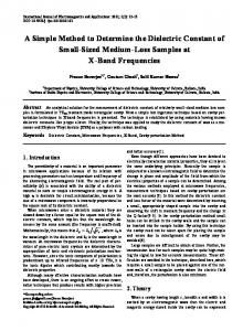
(4) 𝑓𝐴(𝑥) = 𝜔, for 𝑥 ∈ [𝑎2 , 𝑎3 ], where 𝜔 is a constant and 0 < 𝜔 ≤ 1. (5) 𝑓𝐴(𝑥) is strictly decreasing in [𝑎2 , 𝑎3 ]. (6) 𝑓𝐴(𝑥) = 0, for all 𝑥 ∈ [𝑎4 , ∞). Particularly, a trapezoidal fuzzy number and triangular fuzzy number can be shown in Figures 1(a) and 1(b), respectively.

2.4. Generalized Evidence Theory [30]. Generalized evidence theory (GET), based on the classical Dempster-Shafer (DS) theory, was proposed by Deng [30]. GET abolished the restriction on 𝑚(Ø) = 0; that is, 𝑚(Ø) is not necessarily zero. In GET, the empty set (Ø) can be singleton subsets or multiple hypothesis sets. Moreover, GET can degenerate to the classical D-S theory if the value of 𝑚(Ø) is zero. In other words, GET is the extension of the classical D-S theory and can express and deal with more uncertain information in the open world, comparing with D-S theory. 2.4.1. Generalized Basic Probability Assignment [30]. Suppose that 𝑈 is a frame of discernment in an open world [30]. Its 𝑈 power set, 2𝑈 𝐺 , is composed of 2 propositions, ∀𝐴 ⊂ 𝑈. If the 𝑈 function 𝑚 : 2𝐺 → [0, 1] meets the condition ∑ 𝑚𝐺 (𝐴) = 1

𝐴⊆2𝑈 𝐺

then 𝑚𝐺 is the GBPA of the frame of discernment 𝑈. The difference between GBPA and traditional BPA is the restriction of Ø. Note that 𝑚𝐺(Ø) = 0 is not necessary in GBPA. If 𝑚𝐺(Ø) = 0, the GBPA reduces to a traditional BPA. 2.4.2. Generalized Combination Rule (GCR) [30]. In GET, Ø1 ∩ Ø2 = Ø means that the intersection between two empty sets is still an empty set. Given two GPBAs (𝑚1 and 𝑚2 ), the GCR is defined as follows [30]:

̃ is a normal Definition 2 (fuzzy number). A fuzzy number 𝐴 and convex fuzzy subset of 𝑋 [45]. Here, “normality” implies that ⋁𝜇𝐴 ̃ (𝑥) = 1, 𝑥

∃𝑥 ∈ R,

∀𝑥1 ∈ 𝑋, 𝑥2 ∈ 𝑋, ∀𝛼 ∈ [0, 1] .

(2) 𝑓𝐴(𝑥) = 0, for all 𝑥 ∈ (−∞, 𝑎1 ].

(1 − 𝑚 (Ø)) ∑𝐵∩𝐶=𝐴 𝑚1 (𝐵) 𝑚2 (𝐶) 1−𝐾

(13)

𝐾 = ∑ 𝑚1 (𝐵) 𝑚2 (𝐶) , 𝐵∩𝐶=Ø

(14)

𝑚 (Ø) = 𝑚1 (Ø) 𝑚2 (Ø) . (11)

Definition 3 (generalized fuzzy numbers). A generalized fuzzy number 𝐴 = (𝑎1 , 𝑎2 , 𝑎3 , 𝑎4 ; 𝜔) is described as any fuzzy subset of the real line 𝑅 with membership function 𝑓𝐴 that possesses the following features: (1) 𝑓𝐴(𝑥) : 𝑅 → [0, 𝜔] is continuous, 0 ≤ 𝜔 ≤ 1.

𝑚 (𝐴) = with

(10)

and “convex” means that 𝜇𝐴 ̃ (𝛼𝑥1 + (1 − 𝛼) 𝑥2 ) ⩾ min (𝜇𝐴 ̃ (𝑥1 ) , 𝜇𝐴 ̃ (𝑥2 ))

(12)

𝑚(Ø) = 1 if and only if 𝐾 = 1.

3. Proposed Method to Determine BPA Function 3.1. Sample Difference Degree. In order to reflect the difference between the sample and the target model, we proposed a sample difference degree function, which performs well in the measurement of difference between the sample data and

4

Mathematical Problems in Engineering 𝜇A ̃ (x)

𝜇A ̃ (x) ̃ A

1

0

a1

a2

̃ A

1

a3

a4

x

0

a1

a2 = a3

(a)

a4

x

(b)

Figure 1: Trapezoidal and triangular fuzzy number.

the model data. And now, it will be amended to define pessimistic function in a more reasonable way. In our method, the triangular fuzzy numbers, which denote the target model and the sample data, should firstly be ̃ and 𝑎̃0 , respectively. normalized into the interval [0, 1] as 𝐴 Four normalized triangular fuzzy numbers are defined as follows: ̃ = (𝑎, 𝑏, (1) Triangular fuzzy number of target model 𝐴 𝑐; 𝜔). (2) Triangular fuzzy number of sample data 𝑎̃0 = (𝑎0 , 𝑎0 , 𝑎0 ; 1). ̃0 = (0, 0, 0; (3) Left standard triangular fuzzy number 𝐴 1). ̃1 = (1, 1, 1; (4) Right standard triangular fuzzy number 𝐴 1). 𝜔 ∈ [0, 1], 0 ⩽ 𝑎 ⩽ 𝑏 ⩽ 𝑐 ⩽ 1. Then the Left and right ̃ 𝑆L (̃𝑎0 ), 𝑆R (𝐴), ̃ and 𝑆R (̃𝑎0 ), are defined average area, 𝑆L (𝐴), as follows and are shown in Figure 2. As can be seen from ̃ and Figure 2, 𝑔1 (𝑥) is the left membership degree curve of 𝐴, −1 𝑔1 (𝑥) denotes inverse function of 𝑔1 (𝑥); 𝑔2 (𝑥) is the right ̃ and 𝑔−1 (𝑥) denotes inverse membership degree curve of 𝐴, 2 function of 𝑔2 (𝑥). Then the left adjacent area 𝑆LA is the area enclosed by 𝑔1 (𝑥) and left standard triangular fuzzy number (0, 0, 0; 1); the left far area 𝑆LF is the area enclosed by 𝑔2 (𝑥) and left standard triangular fuzzy number (0, 0, 0; 1); the right adjacent area 𝑆RA is the area enclosed by 𝑔2 (𝑥) and right standard triangular fuzzy number (1, 1, 1; 1); the right far area 𝑆RF is the area enclosed by 𝑔1 (𝑥) and right standard triangular fuzzy number (1, 1, 1; 1). Obviously, the four kinds of area can be obtained by the following equations: 𝜔

𝑆LA = ∫ 𝑔1−1 (𝑥) d𝑥, 0 𝜔

SLF = ∫ 𝑔2−1 (𝑥) d𝑥, 0 𝜔

𝑆RA = ∫ (1 − 𝑔2−1 (𝑥)) d𝑥, 0 𝜔

𝑆RF = ∫ (1 − 𝑔1−1 (𝑥)) d𝑥. 0

(15)

Based on the four kinds of area, 𝑆LA , 𝑆LF , 𝑆RA , and 𝑆RF , the left average area 𝑆L and the right average area 𝑆R are defined, respectively, as follows: 𝑆L =

𝑆LA + 𝑆LF , 2

(16)

𝑆R =

𝑆RA + 𝑆RF . 2

(17)

Figure 2 indicates that the larger 𝑆L , the closer the fuzzy ̃ to 𝐴 ̃1 ; the larger 𝑆R , the closer the fuzzy number number 𝐴 ̃ ̃ 𝐴 to 𝐴0 . That is to say, 𝑆L and 𝑆R can accurately represent the position and the state information of a triangular fuzzy number in the interval [0, 1]. Based on the fact that the shape and position of a fuzzy number can, to a large extent, be expressed as the credibility of the proposition, a conclusion can be made that the difference between the average area ̃ 𝑆R (𝐴)) ̃ of 𝐴 ̃ and the average area (𝑆L (̃𝑎0 ), 𝑆R (̃𝑎0 )) of 𝑎̃0 (𝑆L (𝐴), reflects the difference between the sample 𝑎̃0 and the model ̃ So, it is reasonable to define the difference degree dif𝑎 to 𝐴. measure the difference between the sample and the model as follows: 󵄨 ̃ − 𝜔𝑆L (̃𝑎0 )󵄨󵄨󵄨󵄨 + 󵄨󵄨󵄨󵄨𝑆R (𝐴) ̃ − 𝜔𝑆R (̃𝑎0 )󵄨󵄨󵄨󵄨 . (18) dif𝑎 = 󵄨󵄨󵄨󵄨𝑆L (𝐴) 󵄨 󵄨 󵄨 3.2. Frame of Discernment in Open World. According to the basic framework of the generalized evidence theory [30], an open world is absolute and a closed world is relative. Assume the system to be concerned is not complete and the system FOD Θ is constructed as Θ = {𝑎1 , 𝑎2 , . . . , 𝑎𝑛 , Ø}, where Ø denotes the unknown objects. Ø could be one unknown object or the conjunction of several unknown objects. During the procedure of applying GET, new target representation model is generated by machine learning method along with the accumulation of sensor reports to revise the existing target model library until the system is judged to be complete. 3.3. Pessimistic Function. As can be seen from (18), the dif𝑎 reflects the possibility that the sample data may be distributed into the interval built by the training samples. The larger the dif𝑎, the greater the deviation between

Mathematical Problems in Engineering

5

̃ A

𝜔

g1

a

g1

g2

̃0 A

0

̃ A

𝜔

̃0 A

̃1 A

c

b

g2

0

1

a

̃1 A

b

(a) Left adjacent area

a

g1

g2

̃0 A

0

1

g2

̃0 A

̃1 A

c

b

c

̃ A

𝜔

g1

1

(b) Left far area

̃ A

𝜔

c

1

(c) Right adjacent area

0

a

̃1 A

b (d) Right far area

Figure 2: Left and right area between a triangle fuzzy number and standard fuzzy number.

the test sample and the training sample model, and vice versa. From this point of view, we use the dif𝑎 as argument to define a pessimistic function and yield initial BPA, following a pessimistic strategy: when dif𝑎 is greater than a threshold value, the incremental rate of BPA is less than the decreasing rate of dif𝑎; on the contrary, when dif𝑎 is less than the threshold value, the incremental rate of BPA is greater than the decreasing rate of dif𝑎. In this way, pessimistic function can effectively reflect the difference between test sample and training sample models to generate the initial BPA. Definition 4 (pessimistic function). Consider 𝑆 = 𝜔 ⋅ 𝑒−𝑟⋅(dif𝑎/2) ,

(19)

where 𝜔 denotes the height of sample triangular fuzzy number, 𝑟 denotes the difference coefficient, which is used to revise the membership degree of unknown samples, and dif𝑎 denotes the sample difference defined as (18). 3.4. Procedures to Determine BPA. A flow chart of the proposed method is shown in Figure 3 and details are as follows: Consider species 𝑋 = {𝑥1 , 𝑥2 , . . . , 𝑥𝑛 , Ø}, where Ø denotes the unknown elements. Each species 𝑥𝑖 has 𝑘

attributes 𝑥𝑖1 , 𝑥𝑖2 , . . . , 𝑥𝑖𝑘 , so the test sample 𝜉 to be recognized also has 𝑘 attributes 𝜉1 , 𝜉2 , . . . , 𝜉𝑘 . We randomly choose 𝑚 instances for each species 𝑥𝑖 and build the model: 𝑖 𝑇𝑖 = (𝑡1𝑖 , 𝑡2𝑖 , . . . , 𝑡𝑚 ),

(20)

where 𝑇𝑖 is a 𝑘 × 𝑚 matrix and the 𝑗th row 𝑇𝑖 (𝑗, :) denotes 𝑗 attribution value of each sample of species 𝑥𝑖 . 3.4.1. Step 1: Establish the Triangular Fuzzy Number Model ̃𝑖𝑗 = (𝑎𝑖𝑗 , 𝑏𝑖𝑗 , 𝑐𝑖𝑗 ; Matrix. A triangular fuzzy number model 𝐴 1) for 𝑗 attribution of species 𝑥𝑖 is established according to the sample values, where 𝑎𝑖𝑗 = min (𝑇𝑖 (𝑗, :)) , 𝑏𝑖𝑗 =

∑ 𝑇𝑖 (𝑗, :) , 𝑚

(21)

𝑐𝑖𝑗 = max (𝑇𝑖 (𝑗, :)) . Then the triangular fuzzy number models for each attribution ̃𝑖1 , 𝐴 ̃𝑖2 , . . . , 𝐴 ̃𝑖𝑘 ). of species 𝑥𝑖 can be represented as 𝑀𝑖 = (𝐴

6

Mathematical Problems in Engineering

Original dataset

̃ B

̃ A

1

̃ C Training set

Test set

Build the triangular fuzzy number model matrix

𝜔

0

a2 a1 = a3

b1

b3

b2 c1 = c2 c3

1

Figure 4: Generalized fuzzy number yield by two normal fuzzy numbers. Establish the difference matrix of the model

Use the pessimistic function to yield the initial BPA

Calculating the evidence distance

max(d) > 𝜆

Yes

No

BPA conflict resolution

Final BPA

Figure 3: The steps to determine BPA.

Furthermore, all the triangular fuzzy number models for each attribution of species 𝑥𝑖 (𝑖 = 1, 2, . . . , 𝑛) can be acquired and denoted as a 𝑛 × 𝑘 matrix 𝑀 = (𝑀1 , 𝑀2 , . . . , 𝑀𝑛 )󸀠 , where each column of 𝑀 represents the triangular fuzzy numbers belonging to the different species but the same attribution. As can be seen from Figure 4, there is often some intersection between two triangular fuzzy numbers. In most cases, the intersection is a generalized fuzzy number. But in some cases, it is not a generalized fuzzy number, as shown in Figure 4. For this particular case, it can be processed by the method proposed by Xiao et al. [46] to construct a generalized triangular fuzzy number. Besides, if these is no intersection between two fuzzy numbers, a special fuzzy number (0, 0, 0; 0) could be used to represent

this case. To do the same operation on each column of 𝑀, we can get a fuzzy number matrix 𝑀󸀠 = (𝑀1 , 𝑀2 , . . . , 𝑀2𝑛 −1 )󸀠 . The 𝑚th attribution value 𝜉𝑚 (1 ⩽ 𝑚 ⩽ 𝑘) of the test sample 𝜉 to be recognized should be converted to a special triangular fuzzy number ̃𝜉𝑚 = (𝜉𝑚 , 𝜉𝑚 , 𝜉𝑚 ; 1). Doing this processing 𝑘 times, we can get a triangular fuzzy number matrix ̃𝜉 = (̃𝜉1 , ̃𝜉2 , . . . , ̃𝜉𝑘 ). Then 𝑀󸀠 and ̃𝜉 can be merged into a matrix 𝑀𝜉 . Now we need to normalize every triangular fuzzy number of the matrix 𝑀𝜉 to [0, 1]. Each element of the matrix 𝑀𝜉 is divided by 𝑛 times of the maximum element value, where 𝑛 represents normalization coefficient, which is adjustable according to different engineering application. 3.4.2. Step 2: Establish the Differentiation Matrix. In this step, we need to calculate the left and right average area (𝑆L , 𝑆R ) for each triangular fuzzy number in matrix 𝑀𝜉 according to (16) and (17). Based on the area, the sample differentiation matrix dif𝑎 between each of the first 2𝑛 − 1 rows in 𝑀𝜉 and the (2𝑛 − 1) × 𝑘 test sample 𝜉0 could be calculated. 3.4.3. Step 3: Calculate the Similarity Matrix 𝑆. For each element in matrix dif𝑎, a pessimistic function can be defined according to (19): 𝑆 (𝑖, 𝑗) = 𝜔𝑖𝑗 ⋅ 𝑒−𝑟⋅(dif𝑎(𝑖,𝑗)/2) ;

(22)

now we could obtain a similarity matrix 𝑆0 , which denotes the similarity degree between the test sample and the target species models. Assume FOD is incomplete; we first calculate the value of the 𝑗th (𝑗 = 1, 2, . . . , 𝑘) column of matrix 𝑆0 . Then if the result is larger than 1, the 𝑗th column should be normalized and set 𝑆(2𝑛 , 𝑗) = 0 which denotes the similarity degree between the test sample 𝜉0 and Ø; else if the result is less than 1, 𝑆(2𝑛 , 𝑗) = 1 − 𝑆(:, 𝑗) is regarded as the similarity between the test sample 𝜉0 and Ø, where 𝑆(:, 𝑗) represents the sum of the first 2𝑛 − 1 rows in similarity matrix 𝑆0 . Finally, the modified 2𝑛 × 𝑘 similarity matrix 𝑆0 could be regarded as the initial BPA matrix 𝑆2𝑛 ×𝑘 . 3.4.4. Step 4: Calculate Evidence Disctance. Taking each column 𝑆(:, 𝑗) (𝑗 = 1, 2, . . . , 𝑘) in matrix 𝑆2𝑛 ×𝑘 as a piece of evidence or as a vector, we could calculate the distance

Mathematical Problems in Engineering

7

between any two bodies of evidence based on (8) to obtain a distance matrix [𝐷𝑖𝑗 ]𝑘×𝑘 , where 𝐷𝑖𝑗 represents the distance between the 𝑖th and 𝑗th column of the initial BPA matrix 𝑆2𝑛 ×𝑘 . Obviously, 𝐷𝑖𝑗 equals 𝐷𝑗𝑖 ; that is, distance matrix [𝐷𝑖𝑗 ]𝑘×𝑘 is a symmetrical matrix, which can simplify the calculation to a great extent. 3.4.5. Step 5: Determine the Extent of Conflict of Evidence. First, we can sum each row 𝐷(𝑗, :) (𝑗 = 1, 2, . . . , 𝑘) in matrix 𝐷𝑘×𝑘 and obtain a vector 𝑑0 ; it can be normalized as a vector 𝑑 = 𝑑0 / max(𝑑0 ), where max(𝑑0 ) denotes the maximum element of 𝑑0 . As debated in Section 1, classical D-S theory has a vital problem that combining two highly conflicting evidences could get even a wrong result. So a conflict threshold 𝜆 (0 ⩽ 𝜆 ⩽ 1) should be set first according to concrete engineering application. If the maximum element value of vector 𝑑 is less than conflict threshold 𝜆, the conflict degree is acceptable and the initial BPAs could be combined with GCR (see (12) and (13)) directly; otherwise the initial BPAs should be adjusted. The specific process is in Section 3.4.6, with the discount coefficient method. 3.4.6. Step 6: Adjust the Conflicting Evidence by Using the Discount Coefficient Method. This step will be operated if evidence conflict is over threshold 𝜆. In this step, conflict resolution between initial BPAs should firstly be done. Then GCR could be applied to combine the preprocessed BPAs. Computational procedure is summarized as follows: (1) Construct a comparative matrix 𝑃 with the average of each row (𝑑𝑖 ) in distance matrix 𝐷𝑘×𝑘 : 𝑃 (𝑖, 𝑗) =

𝑑𝑖 𝑑𝑗

,

(23)

where 𝑃(𝑖, 𝑗) is the 𝑖th row and 𝑗th column element in matrix 𝑃, 𝑑𝑖 is the 𝑖th row of 𝐷𝑘×𝑘 , and 𝑑𝑗 is the 𝑗th row of 𝐷𝑘×𝑘 . (2) Calculate eigenvector (𝜔𝑖 ) corresponding to the maximum eigenvalue and normalize 𝜔𝑖 as discount coefficient 𝜔. (3) Discount the initial BPAs with coefficient 𝜔 to obtain the final BPAs. (4) Combine the final BPAs with GCR and then the final recognized result will be acquired.

4. Experimental Analysis In this paper, we take Iris dataset [47] to demonstrate the effectiveness of the proposed method. The Iris dataset, which is perhaps the best known database to be found in pattern recognition literature, involves classification of three species of the Iris flowers, Iris setosa (S), Iris versicolour (E), and Iris virginica (V), on the basis of four numeric attributes of the Iris flower: sepal length (SL) in cm, sepal width (SW) in cm, petal length (PL) in cm, and petal width (PW) in cm [47].

In the Iris dataset, there are 50 instances for each of three species. The data are obtained from the UCI repository (UCI Machine Learning Repository: http://archive.ics.uci.edu/ml/ datasets/Iris) of machine learning databases. Among 50 instances of each species, 30 instances are randomly selected as the training set, and the remaining 20 instances serve as the test set. Each of four attributes is regarded as an information source, and correspondingly there are three training sets and three test sets. 4.1. To Recognize Known Species of Iris Dataset. Before the experiment, the fully optimized parameter settings should be obtained first by training the dataset. The conflict threshold 𝜆 can be set according to experts’ experience usually. In this experiment, 𝜆 = 0.2. It means that the conflict is in the acceptable scale only if the maximum conflict between bodies of evidence is less than 0.2. Otherwise the initial BPAs should be adjusted. The difference coefficient 𝑟 can be obtained by an iterative program. The difference coefficient 𝑟 would be adjusted in each iterative step. When the average recognition rate of known species is up to an acceptable scale and the deviation of the average recognition rate between current step and last step was tiny enough, the parameter 𝑟 would be obtained. After the training process, we have obtained the optimized parameter settings as {𝑟 = 12.0, 𝜆 = 0.2}. Because these optimized parameters fit the dataset well, parameters are all set as the optimized settings in the following. Following the steps in Section 3.4, triangular fuzzy numbers of the training samples are built, shown in Table 1 and in Figure 5. According to Step 5 in Section 3.4.5, we can obtain BPAs for each attribute of a Setosa instance (5.1, 3.5, 1.4, 0.2) shown in Table 2. After conflict resolution (if needed), these BPAs in Table 2 could be combined with GCR. The results are as follows: 𝑚 (S) = 0.9655, 𝑚 (E) = 0.0344, 𝑚 (V) = 0.0002, 𝑚 (SE) = 0, 𝑚 (SV) = 0,

(24)

𝑚 (EV) = 0, 𝑚 (SEV) = 0, 𝑚 (Ø) = 0. As can be seen, the combination result illustrates that the test instance (5.1, 3.5, 1.4, 0.2) belongs to species setosa, which is consistent with the actual situation. 4.2. To Recognize Unknown Species of Iris Dataset. In order to check the proposed method’s ability to recognize the unknown species of data in an open world, triangular fuzzy number models are constructed only by two species of Iris dataset selected randomly from the three species this time.

8

Mathematical Problems in Engineering

Table 1: Fuzzy number model constructed by 90 Iris data instances. Item S E V SE SV EV SEV Item S E V SE SV EV SEV

Attributes SL SW (4.4, 4.94, 5.8; 1.0) (3.0, 3.47, 4.0; 1.0) (4.9, 5.48, 6.2; 1.0) (2.0, 2.65, 3.4; 1.0) (6.1, 6.85, 7.7; 1.0) (2.6, 2.94, 3.2; 1.0) (4.9, 5.2625, 5.8; 0.625) (2.0, 2.65, 3.4; 1.0) (0, 0, 0; 0) (2.6, 2.94, 3.2; 1.0) (6.1, 6.151, 6.20; 0.068) (2.6, 2.849, 3.2; 0.733) (0, 0, 0; 0) (2.6, 2.849, 3.2; 0.733) Attributes PL PW (1.0, 1.43, 1.9; 1.0) (0.1, 0.24, 0.6; 1.0) (3.3, 3.9, 4.5; 1.0) (1.0, 1.2, 1.6; 1.0) (4.8, 5.71, 6.7; 1.0) (1.4, 1.99, 2.3; 1.0) (0, 0, 0; 0) (0, 0, 0; 0) (0, 0, 0; 0) (0, 0, 0; 0) (0, 0, 0; 0) (1.4, 1.519, 1.6; 0.202) (0, 0, 0; 0) (0, 0, 0; 0)

Table 2: BPAs for each attribute of a Setosa instance. Item S E V SE SV EV SEV Ø

𝑚 (S) = 0.9629, 𝑚 (E) = 0.0371, 𝑚 (SE) = 0, 𝑚 (Ø) = 0.

(25)

As can be seen, the combination result illustrates that the test instance (4.9, 3.1, 1.4, 0.2) belongs to species setosa. Similarly, to recognize an instance from the open world, we can obtain BPAs for each attribute of a Virginica (V) instance (unknown species) (6.3, 3.3, 6.0, 2.5) in Table 5. As can be seen from Table 5, the difference function dif𝑎 (see (18)) and pessimistic function (see (19)) indeed recognized this instance as a member of species V. After conflict resolution (if needed), these BPAs in Table 5 should be combined again with GCR. The results are as follows: 𝑚 (S) = 0.0009, 𝑚 (E) = 0.3955, 𝑚 (SE) = 0, 𝑚 (Ø) = 0.6036.

(26)

Attributes SW PL 0.1828 0.8279 0.1369 0.1536 0.1579 0.0185 0.1369 0 0.1579 0 0.1138 0 0.1138 0 0 0

PW 0.8321 0.1595 0.0084 0 0 0 0 0

Table 3: Fuzzy number model constructed by 60 Iris data instances. Item S E SE Item

Thus, the remaining species of Iris dataset could be regarded as test sets, which are unknown to the recognition system. For example, we randomly selected 30 instances from Setosa (S) and Versicolour (E), respectively, as training samples to construct triangular fuzzy number model and the remaining 20 instances in each species as test samples. And parameters should also be set as the optimized settings obtained in the training process. The training samples’ triangular fuzzy number model is shown in Table 3. For a known Setosa instance (4.9, 3.1, 1.4, 0.2), we can obtain BPAs for each attribute in Table 4, according to Step 5 in Section 3.4.5. After conflict resolution (if needed), these BPAs in Table 4 should be combined with GCR. The results are as follows:

SL 0.3232 0.2790 0.2104 0.0717 0 0.1157 0 0

S E SE

Attributes SL SW (4.7, 5.19, 5.7; 1.0) (3.1, 3.62, 4.4; 1.0) (5.1, 5.97, 6.7; 1.0) (2.5, 2.84, 3.1; 1.0) (5.1, 5.478, 5.7; 0.4383) (0, 0, 0; 0) Attributes PL PW (1.3, 1.5, 1.7; 1.0) (0.2, 0.28, 0.4; 1.0) (3.0, 4.23, 5.0; 1.0) (1.1, 1.36, 1.7; 1.0) (0, 0, 0; 0) (0, 0, 0; 0) Table 4: BPAs for each attribute of a Setosa instance.

Item S E SE Ø (V)

SL 0.4448 0.3352 0.2200 0

Attributes SW PL 0.3888 0.8036 0.3888 0.1964 0.2224 0 0 0

PW 0.8256 0.1559 0 0.0185

And the recognition result suggests that the test instance (6.3, 3.3, 6.0, 2.5) is an unknown species of Iris datasets. In order to further illustrate the validity and accuracy of the proposed method, the same experiments have been done 100 times. And to be satisfied, the average recognition rate about known-species Iris dataset (in closed world) is up to 81.55% and the average recognition rate about unknownspecies Iris dataset (in open world) is up to 73.40%. Several unrecognized data in one experiment are shown in Table 6. As can be seen from Table 6, two instances of species E were recognized as species V, and two datasets of species V were recognized as species E and Ø (that is, species S), respectively. And two instances of species Ø (species S) were recognized as species E. It is not difficult to explain the wrong results. From Table 1 and Figure 5 we can see that only attributes PL and PW of species setosa are totally separated from species E and species V, and the two remaining attributes are all intersected with others. At the same time, species E and species V intersect with each other for each of attributes. Especially since the length of interval overlapping in the SL and SW attribute

9

1

1

0.8

0.8 Membership function

Membership function

Mathematical Problems in Engineering

0.6

0.4

0.2

0

0.4

0.2

4

4.5

5

5.5

Setosa Versicolor

6 6.5 SL (cm)

7

7.5

0

8

2.25

2.5

2.75

3

Setosa Versicolor

Virginica

1

1

0.8

0.8

0.6

0.4

0.2

0

2

3.25

3.5

3.75

4

3

3.5

4

SW (cm)

Membership function

Membership function

0.6

Virginica

0.6

0.4

0.2

0

1

2

Setosa Versicolor

3

4 PL (cm)

5

6

7

0

8

0

0.5

1

1.5

2 2.5 PW (cm)

Setosa Versicolor

Virginica

Virginica

Figure 5: The fuzzy number representation of each attribute of each species.

Table 5: BPAs for each attribute of a Virginica instance. Item S E SE Ø (V)

SL 0.0118 0.0434 0.0313 0.9136

Attributes SW PL 0.2214 0 0.0188 0.0011 0.0983 0 0.6615 0.9989

PW 0 0.0001 0 0.9999

is large, all the attributes of some data intersect with each other and it is difficult to distinguish these attributes using pessimistic function. Even so, the simulation examples show that the average recognition rate for the instances of the known species is up to 81.55% and the average recognition rate of the unknown-species instances is up to 73.40%. Moreover, during the process of recognition, the number of training samples is small (only 30 instances in each species), and test samples are totally separated from training samples.

Table 6: Unrecognized instances in an experiment. SL 5.9 6.7 7.7 6.1 5.0 5.4

SW 3.2 3.1 2.6 2.6 3.0 3.4

PL 4.8 4.7 6.9 5.6 1.6 1.5

PW 1.8 1.5 2.3 1.4 0.2 0.4

Sample species E E V V Ø Ø

Recognition result V V Ø E E E

It scientifically proves that the proposed method to determine BPA has great effectiveness and could work well with GET.

5. Conclusion In the application of data fusion, the generalized evidence theory (GET) has more advantages than the classical Dempster-Shafer evidence theory due to its ability to deal with evidence conflict when the frame of discernment is

10 incomplete. How to determine the generalized basic probability assignment (GBPA) in an open world is still an open issue. A method to construct GBPA is proposed in this paper. This method uses training samples to build triangular fuzzy number models for each attribute of the multiattribute dataset. Then, the differentiation function and the similarity function are defined. The initial GBPAs are generated by the similarity function, and bodies of evidence are fused with Dempster’s rule or the generalized combination rule (GCR) according to the actual target environment. This method makes full use of the advantages of GET to deal with these targets in the open world. In order to reduce the impact of conflicting evidence on the fusion results, the distance between each body of evidence is calculated and conflict resolution is to be done in the initial stage of determining GBPAs to eliminate human interference and environment noise. Several numerical examples show that the method is concise and effective, and this method has a very significant data processing capacity of small samples based on a good theoretical foundation. The proposed method to obtain GBPA can effectively overcome the problem of subjectivity, which has strong generality. The classification of Iris data is used to illustrate the efficiency and the low computational complexity of the proposed method. This method will help to promote GET and use GCR effectively.

Competing Interests

Mathematical Problems in Engineering

[7]

[8]

[9]

[10]

[11]

[12]

[13]

[14]

The authors declare that there is no conflict of interests regarding the publication of this paper.

Acknowledgments The work is partially supported by National Natural Science Foundation of China (Grant nos. 60904099 and 61501377) and Natural Science Basic Research Plan in Shaanxi Province of China (Program no. 2016JM6018).

References

[15]

[16]

[17]

[1] A. P. Dempster, “Upper and lower probabilities induced by a multivalued mapping,” Annals of Mathematical Statistics, vol. 38, pp. 325–339, 1967.

[18]

[2] G. Shafer, A Mathematical Theory of Evidence, Princeton University Press, New Jersey, NJ, USA, 1976.

[19]

[3] C. Mellish and X. Sun, “The semantic web as a linguistic resource: opportunities for natural language generation,” Knowledge-Based Systems, vol. 19, no. 5, pp. 298–303, 2006. [4] Y.-Z. Liu, Y.-C. Jiang, X. Liu, and S.-L. Yang, “CSMC: a combination strategy for multi-class classification based on multiple association rules,” Knowledge-Based Systems, vol. 21, no. 8, pp. 786–793, 2008. [5] E. Bagheri, R. Zafarani, and M. Barouni-Ebrahimi, “Can reputation migrate? On the propagation of reputation in multi-context communities,” Knowledge-Based Systems, vol. 22, no. 6, pp. 410– 420, 2009. [6] X. Zhao, R. Wang, H. Gu, G. Song, and Y. L. Mo, “Innovative data fusion enabled structural health monitoring approach,”

[20]

[21]

[22]

Mathematical Problems in Engineering, vol. 2014, Article ID 369540, 11 pages, 2014. C. Fu and K.-S. Chin, “Robust evidential reasoning approach with unknown attribute weights,” Knowledge-Based Systems, vol. 59, pp. 9–20, 2014. C. Fu and S. Yang, “An evidential reasoning based consensus model for multiple attribute group decision analysis problems with interval-valued group consensus requirements,” European Journal of Operational Research, vol. 223, no. 1, pp. 167–176, 2012. X. Su, S. Mahadevan, P. Xu, and Y. Deng, “Dependence assessment in human reliability analysis using evidence theory and AHP,” Risk Analysis, vol. 35, no. 7, pp. 1296–1316, 2015. H.-C. Liu, J.-X. You, X.-J. Fan, and Q.-L. Lin, “Failure mode and effects analysis using D numbers and grey relational projection method,” Expert Systems with Applications, vol. 41, no. 10, pp. 4670–4679, 2014. W. Jiang, B. Wei, C. Xie, and D. Zhou, “An evidential sensor fusion method in fault diagnosis,” Advances in Mechanical Engineering, vol. 8, no. 3, pp. 1–7, 2016. W. Jiang, C. Xie, B. Wei, and D. Zhou, “A modified method for risk evaluation in failure modes and effects analysis of aircraft turbine rotor blades,” Advances in Mechanical Engineering, vol. 8, no. 4, pp. 1–16, 2016. F. Lolli, A. Ishizaka, R. Gamberini, B. Rimini, and M. Messori, “FlowSort-GDSS—a novel group multi-criteria decision support system for sorting problems with application to FMEA,” Expert Systems with Applications, vol. 42, no. 17-18, pp. 6342– 6349, 2015. N. Rikhtegar, N. Mansouri, A. A. Oroumieh, A. YazdaniChamzini, E. K. Zavadskas, and S. Kildien˙e, “Environmental impact assessment based on group decision-making methods in mining projects,” Economic Research, vol. 27, no. 1, pp. 378– 392, 2014. D. Niu, Y. Wei, Y. Shi, and H. R. Karimi, “A novel evaluation model for hybrid power system based on vague set and Dempster-Shafer evidence theory,” Mathematical Problems in Engineering, vol. 2012, Article ID 784389, 12 pages, 2012. R. R. Yager, “On the fusion of non-independent belief structures,” International Journal of General Systems, vol. 38, no. 5, pp. 505–531, 2009. X. Su, S. Mahadevan, W. Han, and Y. Deng, “Combining dependent bodies of evidence,” Applied Intelligence, vol. 44, pp. 634–644, 2016. X. Su, S. Mahadevan, P. Xu, and Y. Deng, “Handling of dependence in Dempster-Shafer theory,” International Journal of Intelligent Systems, vol. 30, no. 4, pp. 441–467, 2015. P. D. Xu, X. Y. Su, S. Mahadevan, C. Z. Li, and Y. Deng, “A nonparametric method to determine basic probability assignment for classification problems,” Applied Intelligence, vol. 41, no. 3, pp. 681–693, 2014. D. Suh and J. Yook, “A method to determine basic probability assignment in context awareness of a moving object,” International Journal of Distributed Sensor Networks, vol. 2013, Article ID 972641, 7 pages, 2013. S. Yoon, C.-K. Ryu, and D. Suh, “A novel way of BPA calculation for context inference using sensor signals,” International Journal of Smart Home, vol. 8, no. 1, pp. 1–8, 2014. W. Jiang, Y. Luo, X. Qin, and J. Zhan, “An improved method to rank generalized fuzzy numbers with different left heights and right heights,” Journal of Intelligent and Fuzzy Systems, vol. 28, no. 5, pp. 2343–2355, 2015.

Mathematical Problems in Engineering [23] W. Jiang, Y. Yang, Y. Luo, and X. Qin, “Determining basic probability assignment based on the improved similarity measures of generalized fuzzy numbers,” International Journal of Computers, Communications & Control, vol. 10, no. 3, pp. 333–347, 2015. [24] L. A. Zadeh, “A simple view of the dempter-shafer theory of evidence and its implication for the rule of combination,” AI Magazine, vol. 7, no. 2, pp. 85–90, 1986. [25] C. Yu, J. Yang, D. Yang, X. Ma, and H. Min, “An improved conflicting evidence combination approach based on a new supporting probability distance,” Expert Systems with Applications, vol. 42, no. 12, pp. 5139–5149, 2015. [26] W. Jiang, B. Wei, X. Qin, J. Zhan, and Y. Tang, “Sensor data fusion based on a new conflict measure,” Mathematical Problems in Engineering, Article ID 5769061, 2016. [27] R. R. Yager, “On the Dempster-Shafer framework and new combination rules,” Information Sciences, vol. 41, no. 2, pp. 93– 137, 1987. [28] D. Dubois and H. Prade, “A survey of belief revision and updating rules in various uncertainty models,” International Journal of Intelligent Systems, vol. 9, no. 1, pp. 61–100, 1994. [29] P. Smets and R. Kennes, “The transferable belief model,” Artificial Intelligence, vol. 66, no. 2, pp. 191–234, 1994. [30] Y. Deng, “Generalized evidence theory,” Applied Intelligence, vol. 43, no. 3, pp. 530–543, 2015. [31] Z. Xu and M. Xia, “Induced generalized intuitionistic fuzzy operators,” Knowledge-Based Systems, vol. 24, no. 2, pp. 197–209, 2011. [32] Y. Deng, S. Mahadevan, and D. Zhou, “Vulnerability assessment of physical protection systems: a bio-inspired approach,” International Journal of Unconventional Computing, vol. 11, pp. 227– 243, 2015. [33] J.-B. Yang and D.-L. Xu, “Evidential reasoning rule for evidence combination,” Artificial Intelligence, vol. 205, pp. 1–29, 2013. [34] Y. Yang and D. Han, “A new distance-based total uncertainty measure in the theory of belief functions,” Knowledge-Based Systems, vol. 94, pp. 114–123, 2016. [35] R. R. Yager and N. Alajlan, “Decision making with ordinal payoffs under Dempster-Shafer type uncertainty,” International Journal of Intelligent Systems, vol. 28, no. 11, pp. 1039–1053, 2013. ´ Boss´e, “A new distance [36] A.-L. Jousselme, D. Grenier, and E. between two bodies of evidence,” Information Fusion, vol. 2, no. 2, pp. 91–101, 2001. [37] L. A. Zadeh, “Fuzzy sets,” Information and Computation, vol. 8, pp. 338–353, 1965. [38] G. Fan, D. Zhong, F. Yan, and P. Yue, “A hybrid fuzzy evaluation method for curtain grouting efficiency assessment based on an AHP method extended by D numbers,” Expert Systems with Applications, vol. 44, pp. 289–303, 2016. [39] Y. Deng, “A threat assessment model under uncertain environment,” Mathematical Problems in Engineering, vol. 2015, Article ID 878024, 12 pages, 2015. [40] Y. Deng, “Fuzzy analytical hierarchy process based on canonical representation on fuzzy numbers,” Journal of Computational Analysis and Applications, In press. [41] S.-B. Tsai, M.-F. Chien, Y. Xue et al., “Using the fuzzy DEMATEL to determine environmental performance: a case of printed circuit board industry in Taiwan,” PLoS ONE, vol. 10, no. 6, Article ID e0129153, 2015. [42] A. Mardani, A. Jusoh, and E. K. Zavadskas, “Fuzzy multiple criteria decision-making techniques and applications— two decades review from 1994 to 2014,” Expert Systems with Applications, vol. 42, no. 8, pp. 4126–4148, 2015.

11 [43] C. Changdar, G. S. Mahapatra, and R. K. Pal, “An ant colony optimization approach for binary knapsack problem under fuzziness,” Applied Mathematics and Computation, vol. 223, pp. 243–253, 2013. [44] Y. Deng, Y. Liu, and D. Zhou, “An improved genetic algorithm with initial population strategy for symmetric TSP,” Mathematical Problems in Engineering, vol. 2015, Article ID 212794, 6 pages, 2015. [45] D. Dubois and H. Prade, Fuzzy Sets and Systems: Theory and Applications, Academic Press, New York, NY, USA, 1980. [46] J. Y. Xiao, M. M. Tong, and C. J. Zhu, “Basic probability assignment construction method based on gerneralized triangular fuzzy number,” Journal of Scientific Instrument, vol. 33, pp. 430– 434, 2012. [47] R. A. Fisher, “The use of multiple measurements in taxonomic problems,” Annals of Human Genetics, vol. 7, no. 2, pp. 179–188, 1936.

Advances in

Operations Research Hindawi Publishing Corporation http://www.hindawi.com

Volume 2014

Advances in

Decision Sciences Hindawi Publishing Corporation http://www.hindawi.com

Volume 2014

Journal of

Applied Mathematics

Algebra

Hindawi Publishing Corporation http://www.hindawi.com

Hindawi Publishing Corporation http://www.hindawi.com

Volume 2014

Journal of

Probability and Statistics Volume 2014

The Scientific World Journal Hindawi Publishing Corporation http://www.hindawi.com

Hindawi Publishing Corporation http://www.hindawi.com

Volume 2014

International Journal of

Differential Equations Hindawi Publishing Corporation http://www.hindawi.com

Volume 2014

Volume 2014

Submit your manuscripts at http://www.hindawi.com International Journal of

Advances in

Combinatorics Hindawi Publishing Corporation http://www.hindawi.com

Mathematical Physics Hindawi Publishing Corporation http://www.hindawi.com

Volume 2014

Journal of

Complex Analysis Hindawi Publishing Corporation http://www.hindawi.com

Volume 2014

International Journal of Mathematics and Mathematical Sciences

Mathematical Problems in Engineering

Journal of

Mathematics Hindawi Publishing Corporation http://www.hindawi.com

Volume 2014

Hindawi Publishing Corporation http://www.hindawi.com

Volume 2014

Volume 2014

Hindawi Publishing Corporation http://www.hindawi.com

Volume 2014

Discrete Mathematics

Journal of

Volume 2014

Hindawi Publishing Corporation http://www.hindawi.com

Discrete Dynamics in Nature and Society

Journal of

Function Spaces Hindawi Publishing Corporation http://www.hindawi.com

Abstract and Applied Analysis

Volume 2014

Hindawi Publishing Corporation http://www.hindawi.com

Volume 2014

Hindawi Publishing Corporation http://www.hindawi.com

Volume 2014

International Journal of

Journal of

Stochastic Analysis

Optimization

Hindawi Publishing Corporation http://www.hindawi.com

Hindawi Publishing Corporation http://www.hindawi.com

Volume 2014

Volume 2014