A METHOD TO DETERMINE THE HEIGHT OF THE MIXED LAYER FROM SPECTRAL PEAK FREQUENCY OF HORIZONTAL VELOCITY K. P. R. Vittal Murty*, Gannabathula S. S. D. Prasad*, Leonardo Deane de Abreu Sá, Edson P. Marques Filho* Divisão de Ciências Meteorológicas/INPE (
[email protected]); fax: (012)345.6666 Amaury de Souza Departamento de Física/Universidade Federal do Mato Grosso do Sul (fax: (067)787.3093) Yadvinder Malhi Institute of Ecology and Resource Management /University of Edinburgh
Resumo Neste artigo é apresentado um novo método para determinar a altura da camada de mistura, estimada através do espectro da velocidade horizontal. O espectro da velocidade horizontal foi calculado com os dados obtidos durante o Experimento Interdisciplinar do Pantanal (IPE-1) para dois dias: um de céu claro e outro de céu nublado. A variação diurna da altura da camada de mistura apresentada para os dois dias, mostrou-se mais pronunciada no dia de céu claro se comparado ao dia de céu nublado.
Keywords Micrometeorology, Mixed Layer, Spectra, Pantanal.
1 - Introduction The mixed layer z i is a scale height that characterizes the structure and development of the planetary boundary layer. It plays an important role in the parametrization of the boundary layer in macro-scale and meso-scale numerical simulations. The traditional methods of mixed layer determination are dependent on profiles of wind speed u , potential temperature θ , standard deviation of the vertical wind speed σ w and sodar echo intensity and using tethered balloon as well as air craft. These were used in large scale field experiments but was not applied for small scale micro meteorological experiments with limited resources. However its should be mentioned here that the eddy correlation technique has become routine for determination of fluxes in the surface layer. This paper works out the mixed layer height only from the peak frequency of the velocity spectra in the lines proposed by Liu and Ohtaki (1997).
2 - Methodology The IPE-1 is a part of broad experimental programe to study the weather and climate of central region of Brazil. The data collection campaign was carried out in South Mato Grosso Pantanal in the experimental site in the farm São Bento (19o33S and 53o8W), 1.5km from the Pantanal studies base of UFMS in Passo do Lontra, Miranda, MS. A micro meteorological tower 21m height was installed and a fast response three dimentional sonic anemometer was installed at 25m. Determination of ML (Mixed Layer) height from the peak frequency of horizontal velocity spectra. The spectrum of the vertical velocity component obeys Monin-Obukhov similarity theory quite well in the surface layer because of its distinct spread with stability. In contrast, the horizontal (*) The authors are grateful to CNPq for providing finantial grant.
wind spectral are scaled with z i , due to the effects of the low frequency convective eddies. Nevertheless the spectrum still obeys Monin-Obukhov and Kolmogorov scaling with high frequencies (Kaimal, 1978; Hojstrup, 1982; Panofsky and Dutton, 1984; Stull, 1988). Hojstrup (1982) suggested that the spectral density can be split into low frequency and high frequency portians S(f ) = S L (f ) + S H (f ) (1) where for the horizontal velocity components u , and v the low frequency spectrum SL (f ) depends on normalized frequency n i = fz i u and (z i L ) while high frequency spectrum S H (f ) depends on reduced frequency n = fz u .Here ' f ' is the natural frequency spectrum u mean wind speed and L is the Obukhov lenght. The resulting equations are adjusted to fit the conditions of inertial range and are expressed according to Panofsky and Dutton (1984) fS u (f ) 0.5n i = 5 2 u* 1 + 2.2n i 3
zi − L
2
3
+
105n
(1 + 33n )
5
3
0.95n i z i 3 17n fS v (f ) = − + 5 2 u* (1 + 2n i ) 3 L (1 + 9.5n )5 3
(2)
2
(3)
The highest values of spectral density appear in low frequency range and is assisted with normalized frequency n i = fz i u . Mathematically the position of peak frequency can be obtained by taken differential of (2) or (3) and equating it to zero d [fS (f )] =0 dz i u*2
If we consider the longitudinal velocity spectrum, it reaches maximum at n i max = 0.7974 . This value corresponds to mixed layer height, z i , as z i = 0.7974
{ since
n = fz u
u z = 0.7974 fu max n u max
or u fu max = z n} with similar arguments it can also be shown as z i = 0.75
(4)
z n v max
(5) Thus z i can be estimated from either Eq. (4) or Eq. (5), knowing the peak frequency of horizontal later or longitudinal velocity (n u max or n v max ) respectively. Here z refers the level, where horizontal velocity is measured by fast response sonic anemometer.
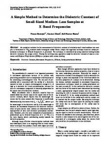
3 - Results and discussion The above theory has been applied to the Pantanal fast response data obtained by a sonic anemometer. The latitudinal and longitudinal velocity spectra were obtained for a cloudy day (julian day 136) and clear day (julian day 143) respectively. Only the spectra with distinct maxima are selected and z i has been estimated. The results were shown in Figs. 1 and 2. Fig. 1 shows the diurnal march of z i for a cloudy day that is julian day 136. It is estimated from both u and v espectra. The depth of mixing layer slowly increased in the morning hours. It is around 800 meters in the evening hours from 18:00 hours and 21:00. Fig 2 represents the z i variation an a clear day. Naturally be expected z i is having more depth and the maximum is around 2000 meters. Better than the longitudinal spectra (u ) the latitudinal spectra (v ) reveals a gradual increase and decrease. It is interesting to note both u, v spectra confirmed an increase in the night time around 21:00 hours. This might be linked to synoptic or mesoscale phenomena.
d ay 136 2000 Z i (u)
1600 1200 800 400 0 0 :0 0
3 :0 0
6 :0 0
9 :0 0
1 2 :0 0 1 5 :0 0 1 8 :0 0 2 1 :0 0 h ours
d ay 136 2000 Z i (v)
1600 1200 800 400 0 0 :0 0
3 :0 0
6 :0 0
9 :0 0
1 2 :0 0 1 5 :0 0 1 8 :0 0 2 1 :0 0 h ours
Fig. 1 - The diurnal march of mixing layer depth for a cloudy day.
Zi (u)
day 143 2400 2000 1600 1200 800 400 0 0:00
3:00
6:00
9:00 12:00 15:00 18:00 21:00 hours
Zi (v)
day 143 2400 2000 1600 1200 800 400 0 0:00
3:00
6:00
9:00 12:00 15:00 18:00 21:00 hours
Fig. 2 - The diurnal march of mixing layer depth for a clear day.
4 - Conclusions (1) The mixed layer depth can be estimated from the horizontal velocity spectra; (2) The mixed layer depth on a cloudy day is less and around 800 meters; (3) The mixed layer is extending upto 2 km. an a clear day in the afternoon hours.
5 - Acknowledgement The authors give thanks for the support received from the Fundação de Amparo à Pesquisa do Estado de São Paulo, FAPESP (proc. no 98/00105-5) and from the Conselho Nacional de Desenvolvimento Científico e Tecnológico, CNPq (procs. nos 381.699/97-8, 381.690/97-0, 139.164/96-0). Acknowledgement is also given to all the people involved in the IPE-1 Project organization and data collecting: Drs. Antônio Ocimar Manzi, Regina Célia dos Santos Alvalá, Clóvis Angeli Sansigolo, Ralf Gielow, Plínio Carlos Alvalá, Clóvis M. do Espirito Santo and Mrs. Paulo Rogério Aquino Arlino, Luis Eduardo Rosa, Celso von Randow, Jorge Martins de Melo, Sabrina B. Monteiro Sambatti, Elizabete Cária Moraes of INPE, Drs. Edson Kassar, Hamilton Germano Pavão, Masao Uetanabaro and Mrs. Carla Muller, Jorge Gonçalves and Waldeir Moreshi Dias of Universidade Federal do Mato Grosso do Sul, Dr. Bart Kruijt of University of Edinburgh, Dr. Maria Lúcia Meirelles of EMBRAPA/CPAC, Dr. Romísio Geraldo Bouhid André of UNESP/Jaboticabal. Special thanks are due also to Dr. Nelson L. Dias of SIMEPAR and Dr. Paulo Henrique Caramori of IAPAR who provided kindly a sonic anemometer and a hygrometer to be used during the IPE-1 campaign.
6 - References Hojstrup, J. . Velocity spectra in the unstable boundary layer. J. Atmospheric Science, v.39, p. 22392248, 1982. Kaimal, J. C. . Horizontal velocity spectra in an unstable surface layer. J. Atmospheric Science, v.35, p. 18-24, 1978. Liu, X.; Ohtaki, E. . An independent method to determine the height of the mixed layer. Boundary-Layer Meteorology, v.85, p. 497-504, 1997. Panofsky, H. A.; Dutton, J. A. Atmospheric turbulence. Models and methods for enginneering applications. Wiley, New York, 397 p .,1984. Stull, R. B. An introduction to boundary layer meteorology. Netherlands, Kluwer Academic Publishers, 1988, 666 p..