A methodological approach for comparing predictive maps derived from statistic-probabilistic methods CNRCNR-IDPA Milano - Italy
S. Sterlacchini(1), J. Blahut(1,2), C. Ballabio(2), M. Masetti(3), A. Sorichetta(3)
Dept. of Geology Milano - Italy (1)
Dept. of Environmental Sciences Milano - Italy
CNR-IDPA, Institute for the Dynamic of Environmental Processes, National Research Council, Piazza della Scienza 1, 20126 Milan, Italy -
[email protected] (2) Department of Environmental Sciences, University of Milano-Bicocca, Piazza della Scienza 1, 20126 Milan, Italy (3) Earth Science Department “Ardito Desio”, University of Milano, via Mangiagalli 34, 20133 Milan, Italy
STUDY AREA
Landslide susceptibility assessment has shown significant improvements in recent years by using indirect statistically-based methods implemented within GIS. Although spatial data analysis techniques are now widely adopted as effective tools for an independent validation of predicted results in post-processing operations (prediction rate curves and areas under curves - AUC), poor attention is often paid to the evaluation of the spatial variability of the predicted results. The relationships between past events and predisposing factors may give us information on the likely spatial distribution of future occurrences. However, it seems that the quality of predicted results does not automatically increase with the number of predisposing factors used in the modeling procedures, and the significance of such conditioning factors is frequently not thoroughly evaluated. This study is aimed at assessing different spatial patterns of predicted values of landslide susceptibility maps with almost similar prediction rate curves and AUCs. Our approach is applied to an alpine environment (Italian Central Alps) where debris flows represent a frequent damaging process. Weights of Evidence modeling technique (a data driven Bayesian method) was applied using ArcSDM (Arc Spatial Data Modeler). The output prediction maps were reclassified in a same way to compare the predicted results: a relative classification, based on the proportion of the area classified as susceptible, was made. The thresholds among different susceptibility classes were put at each 10 % of the study area, classified decreasingly from the highest to the lowest susceptibility values. According to that, we reclassified the susceptibility maps and, after applying Kappa Statistic, Cluster Analysis, and Principal Component Analysis (PCA), we analyzed the spatial variability of the predicted maps. The results have shown great differences within the output spatial patterns of the predicted maps, also within the highest susceptibility predicted class. The study was settled in a Mountain Consortium of Municipalities in Valtellina di Tirano, an area of about 450 km2 located on the Italian Central Alps (Lombardy Region, Northern Italy). The territory is subdivided among 12 municipalities and it has about 29,000 inhabitants (prevalently sited on the bottom of the valley). The elevation of the study area ranges from 350 m a.s.l., up to 3,370 m. a.s.l. Valtellina has a U-shaped valley profile derived from Quaternary glacial activity. The lower part of the valley flanks is covered with glacial, fluvio-glacial, and colluvial deposits of variable thickness. Valtellina has an unenviable history of intense and diffused landsliding. Statistical analysis (Crosta et al., 2003) shows that a large percentage of landslides is represented by rainfall-induced, small size and thickness slides (up to 1.5 m), with volumes ranging from few up to some hundreds cubic metres. Field surveys allow to map mainly shallow soil slips and/or soil slips – debris flows and slumps affecting Quaternary covers. These phenomena remove portions of cultivated areas (one of the most important source of sustenance for people), causing the interruption of transportation corridors and disruptions in inhabited areas, sometimes determining the temporary evacuation of people. The area suffered from intense rainfall and consequent landslides several times in the past. The major events occurred in 1983, 1987 and 2000. The flood and landslides in 1987 caused a lot of fatalities, many of them by fast moving soil slips – debris flows.
Study Area Km
Valtellina di Tirano study area
Study area: the debris flows scarp areas are represented
This study consists of a seven-steps process: Landuse
Geology
Slope
Aspect
Internal Relief
Profile Curvature
Planar Curvature
1. Database preparation (explanatory variables and training points). To predict the locations of future landslides and evaluate these predictions the 1,478 mapped debris-flows scarp areas were compared statistically with seven geo-referenced explanatory variables: geology (7 map units), land use (7), and topography - input as five separate data layers: slope gradient (8), slope aspect (4), internal relief (7, ∆h/625 m2), slope planar (3) and profile (3) curvature obtained from a digital elevation model (DEM). A single value was assigned to each 5-m pixel in each data layer. 2. Random spatial subdivision of the training points in two mutually exclusive subsets (modeling and predictive subsets). At this stage of the research, we decided to divide the training points (1,478 mapped debrisflows scarp areas) in two equal number and mutually exclusive subsets (739 scarps each one) by a random spatial criterion. One group (modeling subset) was used to model a prediction with several levels of susceptibility. Counting landslides in the other group (predictive subset) that fall inside these susceptibility classes yields statistics for assessing prediction reliability of future failures. 3. Application of the Weights of Evidence modeling technique (Bonham-Carter et al., 1988; Agterberg et al., 1989). The Weights of Evidence model uses a log-linear form of the Bayesian probability model and it is based on the concepts of prior and posterior probabilities. The prior probability Pprior that an event {D} occur per unit area is calculated as the total number (or area) of events over the total area. This initial estimate can be later increased or diminished in different areas by the use of available explanatory variables {B}. The method is based on the calculation of positive and negative weights by which the degree of spatial association among events and explanatory variables may be modelled. Other statistics could be automatically calculated by Arc SDM® extension - Spatial Data Modeller (Kemp et al., 2001) as a useful measure of the spatial correlation between explanatory variables and the occurrence of an event (Bonham-Carter, 1994). This modeling technique was applied several times (13) changing the number of the explanatory variables in each experiment. 4. Classification of the predictive maps in 10 classes using an equal-area criterion. To make an evaluation of the goodness-of-fit, of the predictive power of the maps and to apply Kappa Statistic, Cluster Analysis, and Principal Component analysis a pre-processing of the prediction maps was performed. We applied a 10-classes equal area classification so the set of susceptibility classes has the following characteristics: (1) all 10 classes include the same number of pixels and therefore each class covers the same area on the ground (1/10th of the entire study area, about 45 km2); (2) the 1st class is the most hazardous; and (3) it is relatively simple to compare the spatial distribution of the susceptibility classes. Response 1
100,0
METHODOLOGY
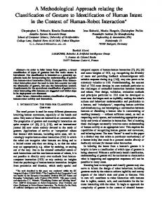
5. Evaluation of the goodness-of-fit using modeling subset (success rate curve). This step is aimed at analysing how well the model fits the occurrences of 739 mapped debrisflows (modeling subsets) in terms of the seven explanatory variables used in each experiment. The degree of fit does not express how well the predictions locate future landslides because the landslides in modeling subset were used to construct the prediction map. Excluding the model nr. 5, the other 12 models seem to fit all equally and well enough the occurrences stored in the modeling subset.
Response 11
Response 13
90,0 Cumulative percentage of landslides within the area classified as hazardous
Response 5
80,0
R_1 70,0
R_2 R_3 R_4
60,0
R_5 R_6
50,0
R_7 R_8
40,0
R_9 R_10
30,0
R_11 R_12
20,0
R_13 10,0
0,0 0,0
10,0
20,0
30,0
40,0
50,0
60,0
70,0
80,0
90,0
100,0
Portion of the study area predicted as hazardous (%)
100,00
Cumulative percentage of landslides within the area classified as hazardous
90,00
6. Evaluation of the predictive power of the maps using predictive subset (by prediction rate curve method, Chung & Fabbri, 2003, 2007). To strength the model prediction the predictive subset was used. A count of landslides in the predictive subset that fall into the susceptibility classes of the prediction map yields prediction rates, which are used here to estimate the reliability and power of the map generated for predicting locations of future landslides. Excluding the predictive map nr. 5, the other 12 predictive maps seem to give all equally the same level of prediction of future landslides.
80,00 R_1 70,00
R_2 R_3
60,00
R_4 R_5 R_6
50,00
R_7 R_8
40,00
R_9 R_10
30,00
R_11 R_12
20,00
R_13 10,00
0,00 0,00
10,00
20,00
30,00
40,00
50,00
60,00
70,00
80,00
90,00
100,00
Portion of the study area predicted as hazardous (%)
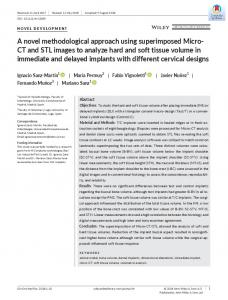
Four of the thirteen predicted maps calculated by the Weights of Evidence modeling technique. Susceptibility classes are represented by a color ramp ranging from warm red (high susceptibility) to dark green (low susceptibility). On each map, the debris flows scarp areas of the predictive subset are superimposed.
Success rate (above) and prediction rate (below) curves of the thirteen experiments
7. Application of Kappa Statistic, Cluster analysis and Principal Component analysis of results. K is a statistical measure of inter-class reliability. It is generally considered a more robust measure than simple percent agreement calculation, since K takes into account the agreement occurring by chance. Cohen's Kappa measures the agreement between two raters, each one classifying N items into C mutually exclusive classes. 1580000
1590000
1595000
1600000
1605000
0.7
Value
0.9
Legend
5140000
0.5
1
5140000
0.6
Value
RMSE Value
-0.2
0.0
2
Comp.2
7
432
-3
-0.6
-2
map5
map9 8 9 map8
Comp.1
5135000 5120000
5125000
5130000
5135000 5130000
5115000
5
0.4
0.6
0.8
-0.6
-0.4
-0.2
0.0
0.2
0.4
0.6
Comp.1
Plotting data within the first two axis of PCA can show how data is clustered in a feature space. In our case the different degree of inter-map class agreement is shown by the proximity of maps within PCA space.
5.000
1580000
1585000
2.500
1590000
0
5.000
1595000
5100000
0.2
5100000
0.0
5105000
4
5105000
-0.4
3 map3 map4
-2
0
map7 map12 map2 10 61 map11 map6 map1
5125000
3 map7 11
map2 map3 map4
5110000
4
0.2
map12
10 9
7 11 2
map6
map9
map1
3
61 8
map11 map9
map5
-0.2
2
5120000
1
2
0.4
6
0.6 0.4
0 map1 map6 map8
5115000
-1
Low : 0
1
-2
map11
map6
-3
6
0
4 5
High : 2,90141
-1
2
0.6
0
0.8
-2
map8
(b) - Classification agreement among Highest susceptibility classes
map3
(a) - Classification agreement among the predicted maps (all classes)
map4
map5 map2
map7
map5 map7
map12
map3
map12
map2
map4
map5
map4
map9
map1
map3
map8
map11
map2
map7
map8
map12
map9
map7
map2
map11
map12
map8
map1
map9
map1
map4
map11
map3
map6
map5
map6
5110000
Very Low Agreement
where P(a) is the relative observed agreement among 0.2 – 0.4 Low Agreement raters, and P(e) is the probability that agreement is due to 0.4 – 0.6 Moderate Agreement chance. If the raters are in complete agreement then K = 1. If there is no agreement among the raters (other than what 0.6 – 0.8 Good Agreement would be expected by chance) then K ≤ 0. For each map 0.8 - 1 Almost perfect Agreement combination the K value was calculated; the results are shown in figure (a) and (b) as heatmaps of the K-values. A cluster analysis performed on the results shows the proximity between different maps. The analysis shows that only 6 maps have a reliable class consistency (with K-values above 0.6). This feature is most striking when compared with the results from prediction rate curves. Excluding Map 5 (which shows a 10 % difference in terms of prediction rate curve) the other maps (all with similar prediction rate values) show levels of proximity really variable (many situations are characterized by low level of inter-class correlation). This means that maps with similar prediction rates could have a different spatial class distribution. Inter-class accuracy increases when only the most susceptible areas are taken into account, as shown in figure (b). This could be seen as a positive result given that an high accuracy for the higher susceptible classes avoids the problem of false negatives. Anyway the inter-maps accuracy is still low for many combinations. A Principal Component Analysis (PCA) was also performed to strength the results abovementioned. PCA can be used for a dimensionality reduction of dataset by retaining those characteristics of the dataset that contribute most to its variance, by keeping lowerorder principal components and ignoring higher-order ones. It is also useful as it can provide a simple way to plot complex multivariate data structures.
FINAL REMARKS
0.2
0.2
0 – 0.2
No Agreement
Comp.2
0
Interpretation
0.0
K
-0.2
P ( a ) − P (e) K= 1 − P ( e)
1585000
Color Key
Color Key
10.000 Meters 1600000
1605000
Root Mean Square Error Map. Debris flows scarp areas are superimposed
Landslide susceptibility maps are essential tools for spatial planning and contributing to public safety worldwide (Guzzetti et al., 1999; Glade et al., 2005). Predictive methods can be based on sophisticated mathematical models operating on complex databases with advanced software and hardware technologies. But potential users may face some problems of interpretation of the predicted information. Some effective approaches to testing the accuracy of the spatial predictions by cross-validation techniques are nowadays available. But, it’s our opinion that when we transpose predicted values from a map to a graph (for evaluating the predictive power of that map) we loose the spatial location of those values. So, two predictive maps with similar predictive power may not have the same meaning. To achieve this aim, we fixed the modeling technique, the number of classes within each explanatory variable, the classification technique, but we changed the number of explanatory variables in each experiment. As we can observe, success-rate curves and prediction-rate curves (excluding the experiment nr. 5) are very similar, testifying for similarities in predictive maps. But the application of Kappa Statistics, Cluster Analysis, and Principal Component Analysis calls for a really different situation.
1