Seungju Yoon, Hainan Li, Jungwook Jun, Jennifer Ogle, Randall Guensler, and Michael Rodgers
1
A Methodology for Developing Transit Bus Speed-Acceleration Matrices to be Used in Load-Based Mobile Source Emissions Models Seungju Yoon Graduate Research Assistant Air Quality Laboratory School of Civil and Environmental Engineering, Georgia Institute of Technology 790 Atlantic Drive Atlanta, GA 30332-0355 TEL: (404) 894-3710 / FAX: (404) 894-9223
[email protected] Hainan Li Graduate Research Assistant School of Civil and Environmental Engineering, Georgia Institute of Technology 790 Atlantic Drive Atlanta, GA 30332-0355
[email protected] Jungwook Jun Graduate Research Assistant School of Civil and Environmental Engineering, Georgia Institute of Technology 790 Atlantic Drive Atlanta, GA 30332-0355
[email protected] Jennifer H. Ogle Research Engineer II School of Civil and Environmental Engineering, Georgia Institute of Technology 790 Atlantic Drive Atlanta, GA 30332-0355
[email protected] Randall L. Guensler Associate Professor School of Civil and Environmental Engineering, Georgia Institute of Technology 790 Atlantic Drive Atlanta, GA 30332-0355 TEL: (404) 894-0405
[email protected] Michael O. Rodgers Principal Research Scientist and Director Air Quality Laboratory School of Civil and Environmental Engineering, Georgia Institute of Technology 790 Atlantic Drive Atlanta, GA 30332-0355 TEL: (404) 894-5609
[email protected] Submitted to: TRB Committee on Transportation and Air Quality (ADC20) in Group D – Planning and Environment Section C – Environment and Energy Date of submittal: November 19, 2004 Word count: 5,206 words (3,706 words in the manuscript + 1,500 for figures)
TRB 2005 Annual Meeting CD-ROM
Paper revised from original submittal.
Seungju Yoon, Hainan Li, Jungwook Jun, Jennifer Ogle, Randall Guensler, and Michael Rodgers
2
ABSTRACT A physical-activity-based transit bus emissions model estimates emissions as a function of transit bus power demand for given transit bus activities and environmental conditions. Transit bus speed and acceleration rates are key activity parameters as well as the most important parameters in the estimation of transit bus power demand, also know as the engine load. Once the transit bus engine load is calculated for a given speed and acceleration, emissions in grams or grams/vehicle-hour can be calculated using grams per brake-horsepower-hour emission rates. To quantify Atlanta regional transit bus speed and acceleration rates, the Georgia Tech research team installed a Georgia Tech Trip Data Collector (consisting of an onboard computer, GPS receiver, a wireless communication device, and data storage) in a transit bus operated by Metropolitan Atlanta Rapid Transit Authority. The team collected second-by-second speed and location data for three weeks, and created speed-acceleration matrices by roadway facility type and by time of day. In this paper, the researchers focused on a methodology development to create transit bus speed-acceleration matrices in use of load-based modal mobile source emissions models for the Atlanta metropolitan area. Once a bus service route is specified by roadway facility type and by time of day, engine power demand for each matrix speed bin can be calculated, weighted by acceleration frequency fractions on each corresponding matrix bin, and then multiplied by emissions levels that can be obtained from engine dynamometer or chassis dynamometer test results.
TRB 2005 Annual Meeting CD-ROM
Paper revised from original submittal.
Seungju Yoon, Hainan Li, Jungwook Jun, Jennifer Ogle, Randall Guensler, and Michael Rodgers
3
INTRODUCTION Since 2000, U.S. Environmental Protection Agency has been developing a new generation mobile source emissions model (Motor Vehicle Emission Simulator, MOVES) based on the specific horsepower requirement of a vehicle. Specific horsepower is a function of speed, acceleration, and road grade (1). In general, a vehicle with higher speed, harder acceleration, and steeper road grade requires more specific horsepower for the vehicle overcome resistance and drag forces. However, collecting speed and acceleration data on various roads during different time periods, and simulating emissions with MOVES would require extensive effort and resources. The Georgia Institute of Technology (Georgia Tech) research team recently developed transit bus speed-acceleration matrices using speed and location data obtained with the Georgia Tech Trip Data Collector having a global positioning system (GPS) receiver. These matrices were designed for use in load-based modal mobile source emissions models. As an emerging vehicle speed data collection tool in transportation research filed, GPS receivers provide accurate speed data calculated based on the Doppler shift theory (2). In studies of vehicle speed accuracy using GPS receivers, vehicle speed from GPS receivers is as accurate as speed obtained from a conventional distance measuring instruments (3) or travel time data acquisition systems (4). Using data from the vehicle speed sensor, researchers validated the GPS speed obtained from the Georgia Tech Trip Data Collector. The GPS receiver provides speed within 0.5 mph of vehicle speed sensor better than 90% of time and within 1 mph better than 99% of the time. The two data streams were highly correlated with an R2 value of 0.998 (5). For this research, the Georgia Tech research team installed a trip data collector on a transit bus operated by Metropolitan Atlanta Rapid Transit Authority (MARTA) and collected second-by-second speed data for three weeks (June 28 to July 17, 2004). Data were collected during all times of vehicle operation on service routes, approaches to service, returns after service, and idling at garages. Transit bus speed and location data collected by GPS and stored on the system remotely transmitted to a Georgia Tech server. From the second-by-second speed data, researchers calculate corresponding second-by-second acceleration. Then, speed and acceleration data are grouped by roadway facility type and by time of day and used to create speed-acceleration matrices, which can be directly applied as inputs in load-based modal mobile source emissions models. With acceleration frequency fractions binned in speed-acceleration matrices, required engine power can be calculated for each matrix cell. For the calculation of emissions rates in grams per hour, calculated required power for each speed-acceleration cell are multiplied by each year’s emissions level in grams per brake-horsepower-hour (bhp-hr), which can be obtained from engine or chassis dynamometer test results by public agencies and university research centers. METHODOLOGY Researchers monitored three weeks of speed and location data for this vehicle as it operated on many different MARTA routes. Only speed data along regular bus service routes during weekdays from valid GPS operation were selected for the generation of speed-acceleration matrices by roadway facility type and by time of day. Through a geographic information systems (GIS) map matching process, roadway facility types (arterials and locals), on which the speed data were collected by the trip data collector, were identified. Speed data for each roadway facility type were grouped by four time periods defined by Atlanta Regional Commission for regional transportation planning purposes (6). The time periods are morning (6
TRB 2005 Annual Meeting CD-ROM
Paper revised from original submittal.
Seungju Yoon, Hainan Li, Jungwook Jun, Jennifer Ogle, Randall Guensler, and Michael Rodgers
4
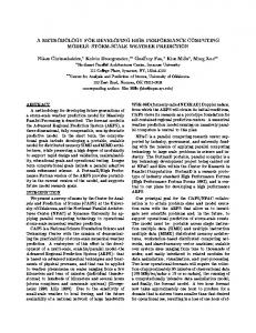
a.m. to 10 a.m.), midday (10 a.m. to 3 p.m.), afternoon (3 p.m. to 7 p.m.), and night (7 p.m. to 6 a.m.) time periods. GPS Antenna Installation Because satellite signals can be blocked by high-story building or overcastting tree canopies, the GPS antenna was installed on the top of the transit bus (Figure 1). It allowed that the GPS antenna received signals from as many satellites as possible. To obtain reliable vehicle speed data, data are only used when the GPS receiver receives a minimum of four satellite signals at the same time (7, 8). In addition, the position dilution of precision (PDOP) value, which is the measure of current satellite geometry, was used to evaluate reliable vehicle speed data. The lower the PDOP value indicates the more accurate GPS positions to get satellite signals. Speed Data Collection and Transmission The Georgia Tech trip data collector consists of four main components: a 386-Linux computer with data storage, a GPS receiver, a wireless communication device, an on-board diagnostic (OBD) data communication device for light-duty vehicles (9). In this study, the light-duty OBD data communication device was disabled. As the transit bus engine is turned on, the trip data collector starts collecting second-by-second speed and location data. Through the wireless communication device, speed and location data were remotely transmitted to a server computer managed by the DRIVE laboratory in the School of Civil and Environmental Engineering at Georgia Tech. Map Matching Process Vehicle position data obtained with the GPS receiver generally do not fall on the center of the GIS digital road links because both the GPS location data and the GIS road links have positional errors from real-world geometric locations. The methodology that places the GPS location data onto the GIS digital road network is called the map-matching. The map-matching process implemented in this study was based on the shortest path function in ArcInfoTM (ESRI) (9). The digital road map used in this study was the Georgia Department of Transportation Digital Linear Graph (DLG) road database. This dataset provides a 1:2,000,000-scale road layer with a full topological structure. The road functional classes from a road characteristic file were spatially joined to the digital road network based on the road characteristics (RC) link ID and mile point information. After the map-matching process, each GPS data point was related to the appropriate road segments in the digital road network and associated to the corresponding road characteristics. In the map-matching process, speed data obtained from the bus moving for more than ten minutes with less than five mph were eliminated to remove bus idling activity at terminals (in some cases, e.g. in New York city, this simplified algorithm might cause the loss of actual onroad operations under extremely congested conditions). Identification of Speed Bins based on GPS Error Because vehicle speed data obtained with a GPS receiver are not as accurate as vehicle speed sensor (VSS) data, the magnitude of error (GPS speed difference from VSS speed) should be evaluated to identify speed bin break points. For instance, if speed error fractions in a speed bin are widely distributed throughout the entire magnitude of error range, it implies that speed obtained with the GPS receiver has significant errors from speed with the VSS. To evaluate the magnitude of error, speed data, which were total 908,088 GPS and VSS paired, were used.
TRB 2005 Annual Meeting CD-ROM
Paper revised from original submittal.
Seungju Yoon, Hainan Li, Jungwook Jun, Jennifer Ogle, Randall Guensler, and Michael Rodgers
5
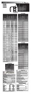
These paired data were obtained from five passenger vehicles equipped with GPS receivers and VSS devices. Speed data were screened based upon the number of satellite channels and PDOP values. Errors of GPS speed dramatically decreased when more than four satellite channels are being received and when PDOP values are less than six. Therefore, speed data obtained with more than four satellite channels and less than six PDOP values were used for the evaluation of the magnitude of error and consisted of 790,037 GPS and VSS light-duty vehicle speed data pairs. Speed bins were arbitrary selected from less than 2.5, 5, 10, 10 to 70 mph, to over 70 mph; speed bins increased with 10 mph interval from 10 to 70 mph. For each speed bin, the fractions of the magnitude of error were plotted with the magnitude of error percentage (Figure 2). For measured speeds less than 5 mph, speed errors were significant and widely distributed. However, at higher speeds, the magnitude of error significantly decreased and narrowed to a ±5% error range. Therefore, the speed range from zero to less than 5 mph was selected as the lowest speed bin. Speed Data Processing To generate speed-acceleration matrices, only speed data on regular bus service routes with valid GPS points during the weekdays were selected. That was because researchers assumed that bus activity (speed and acceleration) on the service routes would differ significantly from the bus activities of leaving or approaching to regular service routes. Due to the data elimination of weak (less than five) satellite signals and high (greater than or equal to six) PDOP values on second-by-second continuous speed data, speed data for analyses became discrete speed data. This may cause inaccurate calculations of acceleration. To avoid the potential errors in acceleration calculation, the first and the last speed and acceleration data in a continuous data block were discarded after acceleration calculation. For the better accuracy and for the lower error of the acceleration calculation, the central difference numerical method was used (11, 12). The central difference numerical method, which adopts two points next to a center point, better reflects the acceleration for the equally spaced speed data. RESULTS AND DISCUSSIONS After the map-matching process, transit bus trips for three weeks were identified on ArcGIS Desktop (ESRI). From transit bus location data, four types of activities were observed: regular bus service (including less than 10-minute idling at terminals), approach for service, return after service, and idling at garages. Among the four types of services, only the regular bus service activity was considered for the speed and acceleration analyses. During the three-week study period, the bus served eleven regular bus routes for more than fifteen vehicle-days in total (Figure 3). The screened data points on the bus service routes provided 229,007 seconds of activity. Among those data points, 64.6% of data were obtained on arterials, 34.2% on locals, and 1.2% on freeways. Relatively few data points were observed on freeways, so that they were excluded from analyses. In total, 226,360 data points (148,039 on arterials and 78,321 on locals) were analyzed to create transit bus speed-acceleration matrices. Speed and Acceleration Characteristics on Arterials Speed on arterials ranged from 0 to 65 mph and acceleration ranged from -9 miles per hour per second (mph/s) to +5 mph/s. The speed and acceleration ranges slightly differed by time of day. In the morning period, speed ranged from 0 to 50 mph and acceleration ranged from -7 to +3 mph/s. Meanwhile speed in the other three time periods covered rather wide ranges from 0 to 65
TRB 2005 Annual Meeting CD-ROM
Paper revised from original submittal.
Seungju Yoon, Hainan Li, Jungwook Jun, Jennifer Ogle, Randall Guensler, and Michael Rodgers
6
mph, and acceleration rates also widely ranged from -9 to +5 mph/s by time period from midday to night. Mean bus speeds increased mildly from morning (15.4 mph), midday (16.0 mph) to afternoon (16.2 mph) time periods. However, the mean speed during the night time period jumped to 19.7 mph. That may be caused by the bus running with lower occupancy in low volume traffic at night, requiring few stops and causing the bus to run faster than the other time periods. The research team plans to investigate this further. Throughout the day, two high acceleration/deceleration peak groups were observed; the first peak group was observed at the speeds less than 5 mph, and the second peak group was observed at the speed range of 20 to 35 mph (Figure 4). The bus accelerated and decelerated frequently at the speed of less than 5 mph (32%, 34%, 37%, and 29% for morning, midday, afternoon, and night time periods). These frequent acceleration and deceleration peaks, ranging from -5 to +3 mph/s, occurred because transit buses frequently stop-and-go at bus stops, intersections, and bus terminals. The second high acceleration/deceleration peak group, which ranges from -9 to +3 mph/s, occurred around the speed range from 20 to 35 mph. These second acceleration/deceleration peaks were equivalent to 35%, 30%, 24%, and 29% of acceleration/deceleration for morning, midday, afternoon, and night time periods. Speed and Acceleration Characteristics on Local Roads Speed on locals roughly ranged from 0 to 45 mph and acceleration ranges from –7 to +5 mph/s. Although occasional high speeds (over 45 mph) were observed on some local roads, their frequencies were less than 2% and were placed in the 45mph bin. Mean bus speeds slightly decreased from morning (14.4 mph), midday (13.8 mph) to afternoon (13.2 mph) time periods. However, the mean speed at night time period jumped to 15.3 mph. The bus ran faster at night than in other time periods. As on arterials, two high acceleration/deceleration peak groups were observed on local roads; the first peak was observed at the speed of less than 5 mph, and the second peak was observed at the speed range of 15 to 30 mph (Figure 5). On local roads, the transit bus most frequently accelerated and decelerated at speeds less than 5 mph (34%, 37%, 40%, and 28% for morning, midday, afternoon, and night time periods). These frequent acceleration and deceleration peaks, which ranged from -6 to +4 mph/s, occurred because the bus frequently stopand-go at bus stops, intersections, and bus terminals. The second high acceleration/deceleration peaks, which ranged from -7 to +5 mph/s, occurred around the speed ranges from 15 to 30 mph. These second acceleration/deceleration peaks were equivalent to 39%, 34%, 28%, and 38% of acceleration/deceleration for morning, midday, afternoon, and night time periods. Speed-Acceleration Matrices and their Applications From the speed and acceleration characteristics, the research team created speed-acceleration matrices by roadway facility type and by time of day. Speed bins ranged from less than 5, 5 to 55, and over 55 mph; speed bins increased with 5 mph interval from 5 to 55 mph. Acceleration bins ranged from less than -10.5, -10.5 to +10.5, and over +10.5 mph/s; acceleration bins increased with 1 mph/s interval from -10.5 to +10.5 mph/s. For the zero acceleration bin, acceleration rates ranged from -0.5 to +0.5 mph/s, which helps to compensate for GPS receiver error. Cells on speed-acceleration matrices were filled with acceleration frequency fractions for corresponding speed and acceleration bins (Figure 6). In the Figure 6, bins of each speed and acceleration interval were filled with median values of its interval. For each roadway facility type and for each time of day, a unique speed-acceleration matrix was created.
TRB 2005 Annual Meeting CD-ROM
Paper revised from original submittal.
Seungju Yoon, Hainan Li, Jungwook Jun, Jennifer Ogle, Randall Guensler, and Michael Rodgers
7
Speed-acceleration matrices generated from transit bus speed data can be directly used to calculate required engine power and then to calculate emissions rates in grams per hour. Once a bus service route is identified by roadway facility type and operation time of day, a proper speedacceleration matrix can be selected. Required engine power for each speed bin in each speedacceleration matrix can be calculated with Equation 1. V ( P=
W a e + FR + FW + FAD + FC ) g 550
(Equation 1)
where, P is the required engine power (bhp) V is the vehicle speed (ft/s) W is the vehicle weight (lbs) a is the vehicle acceleration rates (ft/s2) e is the rotational inertial coefficient (mass factor) FR is the rolling resistance (lbf) FW is the gravitational drag (lbf) FAD is the aerodynamic drag (lbf) FC is the curve resistance (lbf) g is the gravitational force (ft/s2) 550 is the horsepower conversion factor (ft-lbf/s/bhp) Required engine power for each speed bin can be weighted by acceleration frequency fractions on corresponding speed-acceleration bins from each matrix, and the weighted required power will be aggregated as a unique required power for the selected roadway facility type and by time of day. Then, the unique required power can be multiplied by each bus model year emissions level in grams per brake-horsepower-hour, which can be obtained from engine or chassis dynamometer test results by public and university research centers, to calculate an emissions rate in grams per hour for a selected bus service route (Equation 2). Georgia Tech is currently developing a more comprehensive GIS-based, load-based modeling approach for heavy-duty vehicles.
ERi , j =
ELk k
( Pl ,m AFFl , m ) i , j l
(Equation 2)
m
where, ER is the transit bus emissions rate (g/hr) EL is the transit bus emissions level (g/bhp-hr) P is the required engine power (bhp-hr) AFF is the acceleration frequency fraction in a speed-acceleration matrix i is the roadway facility type (Arterial or Local) j is the time of day (Morning, Midday, Afternoon, or Night) k is the engine model year l is the speed in a speed-acceleration matrix m is the acceleration in a speed-acceleration matrix
TRB 2005 Annual Meeting CD-ROM
Paper revised from original submittal.
Seungju Yoon, Hainan Li, Jungwook Jun, Jennifer Ogle, Randall Guensler, and Michael Rodgers
8
To demonstrate emissions rate differences between different speeds with the Equation 2, two cells (7.5 and 37.5 mph at +1 mph/s), which have same acceleration frequency fractions of 0.009, were selected from the Figure 6 (a speed-acceleration matrix for arterials in the morning), and transit bus required power was calculated. Acceleration forces at 7.5 and 37.5 mph were same because acceleration rates were same at those speeds. However, the sum of the other forces (rolling resistance, gravitational drag, and aerodynamic drag) at 37.5 mph was 2.2 times higher than at 7.5 mph. That is because aerodynamic and rolling resistance drag forces increase as vehicle speed increases (13). Required engine power calculated with forces at 37.5 mph was 5.7 times greater than at 7.5 mph; that implies that transit bus emissions rates at 37.5 mph will be 5.7 times greater than at 7.5 mph for +1 mph/s acceleration. CONCLUSIONS AND FUTURE RESEARCH TASKS This research developed transit bus speed-acceleration matrices that are designed to be used in the calculation of load-based modal transit bus emissions rates. Using the Equations 1 and 2 addressed in the previous section, required engine power for each cell on a speed-acceleration matrix can be calculated, weighted by corresponding acceleration frequency fractions, and aggregated as a unique required power for a selected bus service route by time of day. Then, an emissions rate (g/hr) will be calculated with the unique required power multiplied by each bus model year emissions level (g/bhp-hr). These speed acceleration matrices can similarly be used in more complex modal models that require the estimation of second-by-second power demand. The methodology to create speed-acceleration matrices will be further refined with other parameters, such as sub-roadway facility types, hour of day, road grade, vehicle weight, driver behavior, etc. Due to the small size of speed and location data, this paper presents speedacceleration matrices only for two aggregated roadway facility types (arterials and local roads) and four aggregated time periods (morning, midday, afternoon, and night time periods). However, for refined speed-acceleration matrices, arterials and local roads should be subclassified into smaller roadway facility types, and four time periods should be also sub-classified into each hour period. Such matrices can be readily developed for individual transit routes, when instrumented data are collected. With further data collection, speed-acceleration matrices will be incorporated with road grade and vehicle weight because speed and acceleration are functions of required engine power calculation. In general, the steeper road grade and the heavier weight require the greater horsepower for a vehicle overcome resistance forces. With the integration of road grade and vehicle weight, two dimensional speed-acceleration matrices will become multidimensional speed-acceleration matrices for use in load-based modal emissions modeling. In addition, bus drivers’ driving behavior will eventually be investigated and incorporated into the multi-dimensional matrices because different bus drivers may drive a same bus differently. ACKNOWLEDGEMENT Authors express their thanks to Mrs. Sebastian Salontai, William Muckenfuss, and Seyed Mirsajedin, of the Metropolitan Atlanta Rapid Transit Authority, who helped to complete this study. Authors also express their thanks to unidentified bus drivers who drove the bus equipped with a Georgia Tech trip data collector.
TRB 2005 Annual Meeting CD-ROM
Paper revised from original submittal.
Seungju Yoon, Hainan Li, Jungwook Jun, Jennifer Ogle, Randall Guensler, and Michael Rodgers
9
REFERENCES 1. Nam, E. K. Proof of Concept Investigation for the Physical Emission Rate Estimator (PERE) for MOVES. Publication EPA420-R-03-005. EPA, U.S. Environmental Protection Agency, 2003. 2. Hofmann-Wellenhof, B., H. Lichtenegger, and J. Collins. Global Positioning System: Theory and Practice, 3rd Edition. Springer-Verlag Wien, New York, 1994. 3. Ogle, J., R. Guensler, W. Bachman, M. Koutsak, and J. Wolf. Accuracy of Global Positing System for Determining Driver Performance Parameters. In Transportation Research Record: Journal of Transportation Research Board, No. 1818, TRB, National Research Council, Washington, D.C., pp. 12-24 4. D’Este, G., R. Zito, and M. Taylor, Using GPS to Measure Traffic System Performance. Computer-Aided Civil and Infrastructure Engineering, Vol. 14, 1999, pp. 255-265. 5. Jun, J. personal communication of “Reliability of GPS speed data in use of transportation research”, October, 2004 6. Atlanta Regional Commission. Transportation Solutions for a New Century Appendix 4: Model Documentation. October. 23, 2002. 7. Steede-Terry, K. Integrating GIS and the Global Positing System. ESRI Press, California, 2001. 8. Hurn, J. GPS: A Guide to the Next Utility. Trimble, California, 1993. 9. Ogle, J., R. Quantifying Driver Speed Behavior: Estimating Risk through Vehicle Instrumentation. Ph.D. Dissertation, Georgia Institute of Technology, Atlanta, 2004. 10. Li, H. Investing Drivers’ Morning Commute Route Choice Behavior Using Global Positioning Systems Based Multi-day Travel Data. PhD. Thesis. Georgia Institute of Technology, Atlanta, 2005. 11. Burden, R. L., and J. D. Faires. Numerical Analysis, Fourth Edition. PWS-KENT Publishing Company, Boston, 1989. 12. Grant, C. D. Representative vehicle operating mode frequencies: measurement and prediction of vehicle specific freeway modal activity. PhD. Thesis. Georgia Institute of Technology, Atlanta, 1998. 13. Radial Truck Tire & Retread Service Manual. Goodyear Tire & Rubber Company, 2003, pp. 64-79.
TRB 2005 Annual Meeting CD-ROM
Paper revised from original submittal.
Seungju Yoon, Hainan Li, Jungwook Jun, Jennifer Ogle, Randall Guensler, and Michael Rodgers
10
LIST OF FIGURES Figure 1: Georgia Tech Trip Data Collector Installation on a Transit Bus Figure 2: GPS Speed Error Fractions from VSS Speed for Each Speed Bin Figure 3: Speed and Location Data Collected on MARTA Transit Bus Routes Figure 4: Arterial Speed-Acceleration Profiles by Time of Day Figure 5: Local Speed-Acceleration Profiles by Time of Day Figure 6: Example of a Speed-Acceleration Matrix (Arterial, Morning)
TRB 2005 Annual Meeting CD-ROM
Paper revised from original submittal.
Seungju Yoon, Hainan Li, Jungwook Jun, Jennifer Ogle, Randall Guensler, and Michael Rodgers
11
Figure 1: Georgia Tech Trip Data Collector Installation on a Transit Bus
TRB 2005 Annual Meeting CD-ROM
Paper revised from original submittal.
Seungju Yoon, Hainan Li, Jungwook Jun, Jennifer Ogle, Randall Guensler, and Michael Rodgers
12
GPS Speed Error Fractions from VSS Speed for Each Speed Bin
Error Fractions
0
-2 -4 -6 -8 -10 -12 -14 -16 -18 -20
0.00 -0.05 0.10 -0.15 0.20 -0.25 0.30 -0.35 0.40 -0.45 0.50 -0.55 0.60 -0.65 0.70 -0.75 0.80 -0.85 0.90 -0.95 1.00 -1.05 1.10 -1.15 1.20 -1.25 1.30 -1.35 1.40 -1.45 1.50 -1.55
2 4 6 8 + 70 600 5 400 3 200 1 5 5 2. 20
18
16
14
12
10
Magnitude of Error (%)
Speed (mph)
Figure 2: GPS Speed Error Fractions from VSS Speed for Each Speed Bin
TRB 2005 Annual Meeting CD-ROM
Paper revised from original submittal.
0.05 -0.10 0.15 -0.20 0.25 -0.30 0.35 -0.40 0.45 -0.50 0.55 -0.60 0.65 -0.70 0.75 -0.80 0.85 -0.90 0.95 -1.00 1.05 -1.10 1.15 -1.20 1.25 -1.30 1.35 -1.40 1.45 -1.50 1.55 -1.60
Seungju Yoon, Hainan Li, Jungwook Jun, Jennifer Ogle, Randall Guensler, and Michael Rodgers
Figure 3: Speed and Location Data Collected on MARTA Transit Bus Routes
TRB 2005 Annual Meeting CD-ROM
Paper revised from original submittal.
13
Seungju Yoon, Hainan Li, Jungwook Jun, Jennifer Ogle, Randall Guensler, and Michael Rodgers
Transit Bus Speed-Acceleration Profile (Arterial-Morning)
14
Transit Bus Speed-Acceleration Profile (Arterial-Midday) Fraction
Fraction
8 7 5 4 3 2 1 0 -1
-2
-3
-4
-5
-6
-1
1
-9
-8
-7
Acceleration (mph/s)
-1 0
-8 -9 -1 0
-1
1
6
1 7. 0 1 2. 5 2 7.5 5 27 2.5 3 .5 37 2. 5 42 .5 47 . 5 52 .5 .5 55
-1
-2
-3
-4
Speed (mph)
Acceleration (mph/s)
-7
-6
Speed (mph)
-5
0
1
2
3
4
5
6
1 7. 0 1 2. 5 2 7.5 5 27 2.5 3 .5 37 2. 5 42 .5 47 . 5 52 .5 .5 55
7
8
9 10 11
0.09-0.10 0.08-0.09 0.07-0.08 0.06-0.07 0.05-0.06 0.04-0.05 0.03-0.04 0.02-0.03 0.01-0.02 0.00-0.01
9 10 11
0.09-0.10 0.08-0.09 0.07-0.08 0.06-0.07 0.05-0.06 0.04-0.05 0.03-0.04 0.02-0.03 0.01-0.02 0.00-0.01
Transit Bus Speed-Acceleration Profile (Arterial-Afternoon)
Transit Bus Speed-Acceleration Profile (Arterial-Night) Fraction
Fraction
8 7 6 5 4 3 2 1 0 -1
-2
-3
-4
-5
Acceleration (mph/s)
-1
1
-9
-8
-7
-6
Speed (mph)
-1 0
-1
-2
-9 -1 0
-1
1
1 7. 0 1 2. 5 2 7.5 5 27 2.5 3 .5 37 2. 5 42 .5 47 . 5 52 .5 .5 55
-4
-3
Acceleration (mph/s)
-8
-7
-6
Speed (mph)
-5
0
1
2
3
4
5
6
1 7. 0 1 2. 5 2 7.5 5 27 2.5 3 .5 37 2. 5 42 .5 47 . 5 52 .5 .5 55
7
8
9 10 11
0.09-0.10 0.08-0.09 0.07-0.08 0.06-0.07 0.05-0.06 0.04-0.05 0.03-0.04 0.02-0.03 0.01-0.02 0.00-0.01
9 10 11
0.09-0.10 0.08-0.09 0.07-0.08 0.06-0.07 0.05-0.06 0.04-0.05 0.03-0.04 0.02-0.03 0.01-0.02 0.00-0.01
Figure 4: Arterial Speed-Acceleration Profiles by Time of Day
TRB 2005 Annual Meeting CD-ROM
Paper revised from original submittal.
Seungju Yoon, Hainan Li, Jungwook Jun, Jennifer Ogle, Randall Guensler, and Michael Rodgers
Transit Bus Speed-Acceleration Profile (Local-Morning)
15
Transit Bus Speed-Acceleration Profile (Local-Midday) Fraction
Fraction
8 7 5 4 3 2 1 0 -1
-2
-3
-4
-5
-6
-1
1
-9
-8
-7
Acceleration (mph/s)
-1 0
-8 -9 -1 0
-1
1
6
1 7. 0 1 2. 5 2 7.5 5 27 2.5 3 .5 37 2. 5 42 .5 47 . 5 52 .5 .5 55
-1
-2
-3
-4
Speed (mph)
Acceleration (mph/s)
-7
-6
Speed (mph)
-5
0
1
2
3
4
5
6
1 7. 0 1 2. 5 2 7.5 5 27 2.5 3 .5 37 2. 5 42 .5 47 . 5 52 .5 .5 55
7
8
9 10 11
0.09-0.10 0.08-0.09 0.07-0.08 0.06-0.07 0.05-0.06 0.04-0.05 0.03-0.04 0.02-0.03 0.01-0.02 0.00-0.01
9 10 11
0.09-0.10 0.08-0.09 0.07-0.08 0.06-0.07 0.05-0.06 0.04-0.05 0.03-0.04 0.02-0.03 0.01-0.02 0.00-0.01
Transit Bus Speed-Acceleration Profile (Local-Afternoon)
Transit Bus Speed-Acceleration Profile (Local-Night) Fraction
Fraction
8 7 6 5 4 3 2 1 0 -1
-2
-3
-4
-5
Acceleration (mph/s)
-1
1
-9
-8
-7
-6
Speed (mph)
-1 0
-1
-2
-9 -1 0
-1
1
1 7. 0 1 2. 5 2 7.5 5 27 2.5 3 .5 37 2. 5 42 .5 47 . 5 52 .5 .5 55
-4
-3
Acceleration (mph/s)
-8
-7
-6
Speed (mph)
-5
0
1
2
3
4
5
6
1 7. 0 1 2. 5 2 7.5 5 27 2.5 3 .5 37 2. 5 42 .5 47 . 5 52 .5 .5 55
7
8
9 10 11
0.09-0.10 0.08-0.09 0.07-0.08 0.06-0.07 0.05-0.06 0.04-0.05 0.03-0.04 0.02-0.03 0.01-0.02 0.00-0.01
9 10 11
0.09-0.10 0.08-0.09 0.07-0.08 0.06-0.07 0.05-0.06 0.04-0.05 0.03-0.04 0.02-0.03 0.01-0.02 0.00-0.01
Figure 5: Local Speed-Acceleration Profiles by Time of Day
TRB 2005 Annual Meeting CD-ROM
Paper revised from original submittal.
Seungju Yoon, Hainan Li, Jungwook Jun, Jennifer Olge, Randall Guensler, and Michael Rodgers
16
Acceleration (mph/s) Bins
Speed (mph) Bins 0
7.5
12.5
17.5
22.5
27.5
32.5
37.5
42.5
47.5
52.5
55
-11
-
-
-
-
-
-
-
-
-
-
-
-
-10
-
-
-
-
-
-
-
-
-
-
-
-
-9
-
-
-
-
-
-
-
-
-
-
-
-
-8
-
-
-
-
-
-
-
-
-
-
-
-
-7
-
-
-
-
-
-
-
-
-
-
-
-
-6
-
-
-
-
-
-
-
-
-
-
-
-
-5
-
0.001
0.001
0.001
0.001
-
-
-
-
-
-
-
-4
0.002
0.005
0.004
0.003
0.002
0.001
-
-
-
-
-
-
-3
0.005
0.008
0.008
0.008
0.006
0.003
0.002
-
-
-
-
-
-2
0.011
0.007
0.011
0.011
0.008
0.006
0.002
0.001
-
-
-
-
-1
0.019
0.006
0.008
0.013
0.015
0.017
0.011
0.006
0.002
-
-
-
0
0.243
0.008
0.012
0.019
0.045
0.071
0.054
0.028
0.009
0.001
-
-
1
0.024
0.009
0.018
0.030
0.032
0.032
0.019
0.009
0.002
-
-
-
2
0.019
0.023
0.022
0.020
0.013
0.004
0.001
-
-
-
-
-
3
-
0.006
0.005
0.002
0.001
-
-
-
-
-
-
-
4
-
-
-
-
-
-
-
-
-
-
-
-
5
-
-
-
-
-
-
-
-
-
-
-
-
6
-
-
-
-
-
-
-
-
-
-
-
-
7
-
-
-
-
-
-
-
-
-
-
-
-
8
-
-
-
-
-
-
-
-
-
-
-
-
9
-
-
-
-
-
-
-
-
-
-
-
-
10
-
-
-
-
-
-
-
-
-
-
-
-
11
-
-
-
-
-
-
-
-
-
-
-
-
Figure 6: Example of a Speed-Acceleration Matrix (Arterial, Morning)
TRB 2005 Annual Meeting CD-ROM
Paper revised from original submittal.