Satyandra K. Gupta,a Dana S. Nau,b William C. Regli,b and Guangming ... As described in Section 3, an FBM is basically a set of machining features that.
In Jami Shah, Martti Mantyla, and Dana Nau, editors, Advances in Feature Based Manufacturing, Elsevier/North Holland, 1994, pp. 161-184.
A methodology for systematic generation and evaluation of � alternative operation plans Satyandra K. Gupta,a Dana S. Nau,b William C. Regli,b and Guangming Zhanga a Mechanical Engineering Department and Institute for Systems Research, University of Maryland, College Park, MD 20742, USA b Computer Science Department and Institute for Systems Research, University
of Maryland, College Park, MD 20742, USA
Abstract
This chapter describes a methodology for analyzing some of the manufacturability aspects of machined parts during the design stage of the product development cycle, so that problems related to machining can be recognized and corrected while the product is being designed. Starting with the CAD design for a proposed part, our basic approach is to systematically generate alternative operation plans for machining the part, evaluating the capabilities of each operation plan to see which one best balances the need for e�cient manufacturing against the need for a quality product. We anticipate that the information provided by this analysis will be useful both to provide information to the manufacturing engineer about alternative ways in which the part might be machined, and also to give feedback to the designer about problems that might arise with the machining.
1. INTRODUCTION One of the missing links between CAD and CAM is the virtual absence of any systematic methodology for generating and evaluating the alternative ways to manufacture a proposed design. Most integrated CAD/CAM systems try to generate a single process plan for a given design|but in general, there may be several alternative ways to manufacture the design. How easy it is to manufacture|or whether it is even possible to manufacture it at all|may depend on which alternative is chosen. Thus, these alternatives should be generated and examined, to determine how well each one balances the need for a quality product against the need for e�cient manufacturing. In this chapter we describe a methodology for systematically generating and evaluating alternative operation plans for machined parts. Our approach involves representing This work was supported in part by NSF Grants NSFD CDR-88003012, IRI-8907890, and DDM9201779. �
1
the design as a collection of machining features, volumetric features that correspond to machining operations. In general, there may be several alternative representations of the design as di�erent collections of machinable features, corresponding to di�erent ways to machine the part. The basic idea is to generate alternative interpretations of the part as collections of machinable features, map these interpretations into operation plans, and evaluate the manufacturability of each operation plan. More speci cally, our approach involves the following steps: 1. Build the set of all potential machining features F by identifying various features which can be used to create the part P from the stock S , as described in Section 4. Each feature in F represents a di�erent possible machining operation which can be used to create various surfaces of the part. 2. Do the following steps repeatedly, until every promising feature-based model (FBM) for P has been examined: (a) Generate a promising FBM F from the feature set F , as described in Section 5. As described in Section 3, an FBM is basically a set of machining features that contains no redundant features and is su�cient to create the part P . We consider an FBM unpromising if it is not expected to result in any operation plans better than the ones which has already been examined. (b) Do the following steps repeatedly, until every promising operation plan resulting from F has been examined: i. Generate a promising operation plan O from F , as described in Section 6. O represents a partially ordered set of machining operations. We consider an operation plan to be unpromising if it violates any common machining practices. ii. Estimate the achievable machining accuracy of the operation plan O, as described in Section 7.1. If the operation plan O cannot produce the required design tolerances and surface nishes, then discard it and go to Step i. iii. Estimate the production time and cost associated with operation plan O, as described in Section 7.2. 3. If no promising operation plans were found during the above steps, then exit with failure. Otherwise exit with success, returning the operation plan that represents the best tradeo� among quality, cost, and time, as described in Section 7.3. The results of such an analysis can potentially be used for two purposes: (1) to give the production engineer information about what processes and process parameters are most desirable over the various ways in which the part might be machined; and (2) to give the product designer a better understanding of whether and how the design might be changed to improve its manufacturability.
2
2. RELATED WORK Feature-based approaches have been very popular in a variety of CAD/CAM implementations, but di�erent people have used the term to mean di�erent things [27, 9, 14, 6]. Signi cant amounts of work have been directed towards de ning sets of form features to serve as a communication medium between design and manufacturing|but at present, most researchers are convinced that a single set of features cannot satisfy the requirements of both of these domains. The recent trend seems to be toward de ning sets of features with speci c application domains in mind (such as machining, assembly, inspection, etc.). For the machining domain, most researchers agree that volumetric features are preferable to surface features, although certain additional information about the surfaces is needed (for example, to determine accessibility and tool approach directions).
2.1 Recognizing Machining Features
There are three primary approaches for obtaining features from a CAD model. In human-supervised feature recognition, a human user examines an existing CAD model to determine what the manufacturing features are [1]. In automatic feature recognition, the same feature recognition task is performed by a computer system [4, 29, 25, 5, 11, 23]. In design by features, the designer speci es the initial CAD model in terms of various form features which translate directly into the relevant manufacturing features [26, 28, 10]. Many examples exist of each of these approaches. However, these approaches typically produce a single set of features describing the CAD model, rather than several alternative interpretations of the model.
2.2 Generating Alternatives
Hummel [9] and Mantyla [16] present examples of multiple feature representations of the same object. However, these papers do not describe a system or methodology for generating multiple feature models. Hayes's machinist system [8] can identify certain cases in which one feature needs to be made before another. However, its representation of features is not adequate for all aspects of process planning. For example, if it decides that some hole needs to be made before some slot, it does not automatically update the dimensions of the hole or the slot|information which would be needed for process selection. The AMPS process planning system [2] includes a step called \feature re nement," which involves combining a set of features into a more complex feature if it appears that this will optimize the plan, or splitting a feature that cannot be machined into two or more features that can (hopefully) be machined. The techniques for deciding when to combine or split features are heuristic in nature, so from the author's description it is not always clear when alternative interpretations will be produced. Vandenbrande [29] has developed a system that combines techniques from arti cial intelligence and solid modeling. It uses hints or clues to identify potential features in the boundary representation of the part. It is capable of identifying interacting features (e.g., two intersecting slots), and produces alternative feature interpretations in certain cases. The rst systematic work on generation of alternative interpretations was done by Karinthi and Nau [12, 13]. They describe an approach for producing alternative inter3
pretations of the same object as di�erent collections of machining features as the result of algebraic operations on the features, and a system for generating alternative interpretations by performing these algebraic operations. This system works with abstract volumetric features. There is no direct relation between these features and machining operations. Therefore some of the interpretations generated by this approach are not feasible from the machining point of view. In this approach a set of algebraic operators (such as maximal extension, truncation etc.) has been used to generate new interpretations of the part. But this set of operators is not su�cient to generate all interpretations of the part. Moreover, many times the resulting features do not belong to any of the feature classes. Some of the feature interactions may also result in partial ordering among features, which is an important issue from a machining point of view|but this work does not deal with time orderings among the features.
2.3 Evaluating Operation Plans
Because of the need for quality assurance on the shop oor, extensive research has been done on di�erent aspects of evaluation of operation plans. Much of the data relevant for machining operation planning is available in machining data handbooks such as [15]. In addition, mechanistic models have been developed to provide quantitative mappings between machining parameters (such as cutting speed, feed, and depth of cut), to the performance measures of interest (such as surface nish and dimensional accuracy) [7, 2, 35, 36, 30]. Research on machining economics has produced quantitative models for evaluating times and costs related to machining operations [37, 32, 31], and optimization techniques have been applied to these quantitative models to seek the machining parameters which minimize the variable cost, or maximize the production rate and pro t rate associated with machining operations.
3. DEFINITIONS 3.1 Geometric Solids and Machined Parts
For our purposes, a solid is any regular, semi-analytic subset of three-dimensional Euclidean space. If R is any solid, then b(R) is the boundary of R, and �(R) is the interior of R. Note that R = �(R) [ b(R) and that �(R) \ b(R) = ;. If R and R0 are solids, then � 0 0 0 R \ R is the regularized intersection of R and R , i.e., the closure of �(R) \ �(R ). Similarly, � 0 � 0 R [ R and R ? R are the regularized union and regularized di�erence, respectively. For further details on these and other related concepts, see [24]. A machined part (or just a part) is the nished component P to be produced as a result of a sequence of machining operations on a piece of stock S , which is the raw material from which the part is to be machined. The delta volume is the volume to be machined, i.e., � = S ?� P . The workpiece is the intermediate part W produced by performing one or more of the machining operations in the sequence. We will represent P , S , and W as geometric solids.
3.2 Machining Features
In a machining operation, material is removed by relative motion between the cutting tool and the workpiece. The cutting tool is mounted on a large machine tool, and the 4
connected to machine tool
cutting surface datum point (pd)
approach plane
approach face (a(f))
removal volume (rem(f))
trajectory (t) (a) drilling tool (T)
(b) T after rotational sweep (Tv)
accessibility volume (acc(f))
(c) tool swept volume (Tsv)
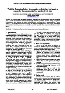
Figure 1: A drilling tool, and the resulting swept volume. total volume occupied by the cutting tool and the machine tool is quite large. But we will only be interested in some small portion of this total volume, namely the portion that actually gets close to the workpiece. We will call this portion the tool volume, and we will denote it by T . Fig. 1(a) shows a drilling tool. To perform a cutting operation, the tool volume T is given a relative cutting motion with respect to the workpiece. This cutting motion may either be imparted to the tool (examples include various milling operations) or the workpiece (examples include various lathe operations). Most of the time this relative cutting motion is either linear (operations such as shaping, planning, broaching) or rotational (operations such as turning, drilling, boring, milling). We represent this motion as a sweep sv which is either linear or rotational. Let Tv denote the solid generated by applying sweep sv to the solid T . For the purpose of locating the tool, we choose a particular point pd of Tv as a datum point. Fig. 1(b) shows Tv and pd for drilling operations. For our purposes, a machining feature is the portion of the workpiece a�ected by a machining operation. However, we will need to know not just the volume of material which the feature can remove from the workpiece, but also what kind of machining operation we are performing, and how we access the workpiece in order to perform the operation. More formally, a machining feature is a triple f = (rem(f ); acc(f ); class(f )), where rem(f ), acc(f ), and class(f ) are as de ned below:
� To perform the machining operation, one sweeps the volume Tv along some tra-
jectory t. The trajectory t is feasible only if sweeping Tv along t does not cause 5
v
v e2
pd
e8
e11 e10
e1 pd
e9
e7 e6
e3
e5
l
l
e4
d
edge loop e = [e1 e2 e3 e4 e5 e6 e7 e8 e9 e10 e11]
(a) a drilling feature (b) a milling feature Figure 2: Examples of machining features
interference problems between the non-cutting surface of Tv and the workpiece. Fig. 1(b) shows an example of a feasible tool trajectory for drilling. If t is feasible, then the solid created by sweeping Tv is Tsv = f(p ? pd ) + q : p 2 T and q 2 tg, as shown in Fig. 1(c). However, only a portion of Tsv actually corresponds to the volume that can be removed by the machining feature. Let the approach surface � be a surface touching solid Tv and containing Tv to one of its sides. This surface is either a plane or a cylinder depending upon the machining operation. For drilling operations this surface is planar as shown in Fig. 1(b). The side containing Tv is called accessibility side. The other side is called removal side. The approach face of f is de ned as a(f ) = � \ Tsv . The removal volume of f is the solid rem(f ) consisting of all points in Tsv that are on the removal side of �. The e�ective removal volume of f is the intersection between rem(f ) and the delta volume; i.e., it is the solid rem(f ) \� �. � The accessibility volume for f is the solid acc(f ) consisting of all points in Tsv that are on the accessibility side of �. � The feature f will be an instance of some feature class �. The feature class � is a parameterized set of machining features corresponding to some machining operation o, and it is characterized by the shape and trajectory of the cutting tool used to perform the operation o. If f is a feature in �, then the class of f is class(f ) = �, and the machining operation for f is op(f ) = o.1 If f is an instance of �, then the f 's parameters in � are the speci c set of parameter values for � that yield f . Below are two examples: In order to create a feature, sometimes we will need several machining operations: a roughing operation followed by one or more nishing operations. In this chapter, we do not handle such cases; instead, we assume that each feature can be made using a single machining operation op( ). This restriction signi cantly limits the scope of the current work, but we intend to remove this restriction in our future work. We believe that it will be relatively straightforward to do so, by using techniques similar to those we employed in our previous work on process selection for roughing and nishing operations [17]. 1
f
f
6
(a) Isometric view (b) Sectioned view (c) FBM 1 (d) FBM 2 Figure 3: A simple part, and two FBMs for it. Note that in FBM 1, the pocket must be made before the hole, and in FBM 2, the hole must be made before the pocket.
{ If we are interested in drilling holes, then we may de ne �d to be the set of all
features that can be created by sweeping a drilling tool of diameter d along a linear trajectory starting at the datum point pd and going in along some unit vector ~v for some distance l. Thus, we can specify a particular feature in �h by giving speci c values for pd , ~v, d, and l. { If we are interested in making milled pockets, slots or faces, then we may de ne �m to be the set of all features that can be created by sweeping a milling tool of radius r in plane, whose parameters are the starting point pd , the depth l, the edge loop e, and the unit orientation vector ~ v. Thus, we can specify a particular feature in �m by giving speci c values for pd, ~v, e, and l. Fig. 2 gives some examples of machining features. A feature f is accessible in a workpiece W if the following conditions are satis ed: 1. f 's accessibility volume does not intersect the workpiece, i.e., acc(f ) \� W = ;. 2. If f 's class is drilling, then to ensure proper machining, the hole's entry face should be a planar surface perpendicular to the hole's axis (no similar condition is needed for milling).
3.3 Feature-Based Models
Depending upon available manufacturing facilities, we will have some xed nite set of feature classes � = f�1; : : : ; �ng, and for each part that we want to manufacture, we will be interested in describing the part in terms of features from �. Suppose we are given a part P and stock S . A feature-based model (or FBM) of P and S is any set of features F having the following properties: 1. Each f 2 F is an instance of some feature class in �. 2. If we subtract the features in F from S , we get P ; i.e. , S ?� Sf 2F rem(f ) = P . 3. No feature in F is redundant, i.e. , for every feature f 2 F; S ?�Sg2F ?ff g rem(g) 6= P . 7
s2 h s1
B
A .01 A
B
Figure 4: An example of a datum-dependency precedence constraint. In this case, s1 should be made before h. For example, Fig. 3 shows a simple part and two FBMs for it. Intuitively, an FBM is an interpretation of the delta volume as a set of machining features. Let f and f 0 be any two distinct features in some FBM. Then f and f 0 intersect each other if rem(f ) \� rem(f 0) 6= ;.
3.4 Precedence Constraints and Operation Plans
Due to accessibility [18], setup [8] and other types of interactions [20] among the features in an FBM F , the features of F cannot be machined in any arbitrary order. Instead, these interactions will introduce precedence constraints requiring that some features of F be machined before or after other features. Let F be an FBM, and let f and f 0 be any two features in F . We will be interested in the following two types of precedence constraints among f and f 0: 1. Accessibility precedence constraint. If acc(f ) \� rem(f 0) 6= ;, then this means that the cutting tool approaches f through the volume occupied by f 0, and thus f 0 must be machined before f . An example is shown in Fig. 3(c), in which the pocket must be machined before the hole. 2. Minimality precedence constraint. Suppose that machining f 0 before f would allow us to machine rem(f ) using a smaller feature g of the same class as f , then we constrain f to be machined before f 0 (for otherwise, we would be machining g rather than f ). An example is shown in Fig. 3(d), in which we would constrain the hole to be machined before the pocket. 3. Datum-dependency precedence constraint. If feature f creates the datum surface for feature g, then f should be machined before g. An example is shown in Fig. 4. If the precedence constraints contradict each other (i.e., if there is no total ordering consistent with them), then we consider F to be unmachinable. Otherwise, the precedence constraints will induce a partial order � on the features of F (i.e., f � f 0 if f must be machined before f 0)|or equivalently, they will induce a partial order on the machining 8
Table 1 Surfaces created by drilling and milling Bottom Side drilling conical (concave) cylindrical (concave) milling planar cylindrical or planar operations corresponding to the features in F (i.e., op(f ) � op(f 0) i� f � f 0). In this case, the operation plan for F consists of the set of machining operations O along with the partial ordering �. Note that every total ordering fo1; o2; : : : ; ok g of O that is consistent with the operation plan will satisfy the following conditions: For each i, let fi be the feature corresponding to oi . Let W0 = S , and Wi = � Wi?1 ? rem(fi ) for all i > 0. Then Condition 1: for all i > 0, fi is accessible in Wi?1, i.e., acc(fi ) \� Wi?1 = ;. Condition 2: each fi is the smallest feature in its class that can be used to produce Wi from Wi?1; i.e., there is no feature f 2 class(fi) such that rem(f ) � rem(fi) and Wi?1 ?� rem(fi) = Wi?1 ?� rem(f ).
4. IDENTIFYING MACHINING FEATURES Given solids representing the part P and the stock S , and a set of feature classes �, we are interested in nding the set F of all features from � that correspond to machining operations that can be used to create P . Each machining feature is capable of creating certain types of surfaces. For example, Table 1 presents the types of surfaces that can be created by drilling (shown in Fig. 2(a)) and milling (shown in Fig. 2(b)). In our approach, we consider all the part surfaces that need to be created, and try to identify features (i.e., instances of feature classes) which are capable of creating those surfaces. The basic idea behind our approach is given below: Let U = b(P ) ?� b(S ) be the set of all faces of P that are not faces of S . These are the faces of P that will need to be machined. For each face u 2 U , do the following: For each feature class � 2 �, add to F every feature f 2 � that has the following properties: 1. f can create u (i.e., u is a subface of some face of f ), and f does not intersect the part (i.e., P \� rem(f ) = ;), 2. for every feature g 2 � that has property 1 and contains f , f and g have the same e�ective removal volume. 3. for every feature g 2 � that has property 1 and is contained by f , g has a smaller e�ective removal volume. 9
Figure 5: Examples of parts recognizable by our feature recognition algorithm. As a speci c instance of this approach, we have developed an algorithm for identifying machining features from a given portion of the boundary of the feature. For the details of the algorithm, readers are referred to [23, 22]. This algorithm handles a large variety of features that correspond to drilling and milling operations, and it is provably complete, even if the features intersect with each other in arbitrarily complex ways. The primary limitation of this algorithm is that it is designed only to handle linearly swept features (i.e., holes, slots, pockets etc.). However, our de nitions of drilling and milling features are more general than the de nitions used in a number of feature recognition systems; for example, milled pockets may be complicated swept contours that include corner radii, islands and other characteristics, in order to realistically describe a non-trivial set of mechanical parts. For example, the algorithm can handle each of the objects shown in Fig. 5. As an example, consider the part shown in Fig. 6. Let us assume that this part will be machined from a rectangular stock made of plain carbon steel (100 BHN), measuring 80mm � 80mm � 55mm. Suppose that the only available feature classes are the class of all drilling features and the class of all milling features. Then Fig. 7 shows the features identi ed by our algorithm.
5. GENERATING FEATURE-BASED MODELS After nding the set of features F , the next step is to use these features to generate FBMs for P and S . Since each FBM is basically an irredundant set cover for the set F , we will generate irredundant FBMs using irredundant-set-covering techniques [21, 19], and use pruning heuristics to discard unpromising FBMs.
Discarding Unpromising FBMs. Let F be an FBM, and let Ls (F ) be the cardinality of the set f~v(f ) : f 2 F g, where ~v(f ) is the unit orientation vector for feature f . Then 10
u1 80 u2
u5
u4
45
o
0.05 A
o
45
0.20 A
0.20 A
11
Figure 6: An example part.
u6 u3 20 30
20 +0.15
20-0.15
50 5
10 10
20
30 55 +0.25
10-0.00 10 80
30
� = fdrilling features,milling featuresg s1
s1’
s3
s2
s4
s4’
s5
s5’
h
F = fs1; s10; s2; s3; s4; s40 ; s5; s50; h; h0g
h’
Figure 7: Features identi ed by our algorithm for the part shown in Fig. 6. 12
FBM1 = fh; s1; s2; s3; s4; s5g:
FBM2 = fh; s1; s2; s3; s40; s50g:
Figure 8: FBMs generated by our algorithm. ( ) is the number of di�erent directions of approach needed in order to machine F , and (except on 5-axis machines or special purpose xtures) is a lower bound on the number of setups needed to machine F . Similarly, let Ltc(F ) be the cardinality of the set f(tool(f ); ~v(f )) : f 2 F g, where tool(f ) is the tool associated with feature f . Then Ltc (F ) is a lower bound on the number of tool changes needed in order to machine F . If two FBMs F and F 0 have same sets of removal volumes but di�erent sets of accessibility volumes, then the expected machining accuracy of F and F 0 is same, but the number of setups and/or tool changes might be di�erent. In this case, we consider F 0 unpromising if either of the following conditions is satis ed: � Ls (F ) � Ls (F 0) and Ltc(F ) < Ltc(F 0), i.e., F is believed to require no more setups than F 0, and fewer tool changes; � Ltc(F ) � Ltc (F 0) and Ls (F ) < Ls (F 0), i.e., F is believed to require no more tool changes than F 0, and fewer setups. As an example, Fig. 8 shows two of the FBMs generated from the features shown in Fig. 7.
Ls F
13
6. GENERATING OPERATION PLANS After generating FBMs, the next step is to generate the associated machining operations along with their partial orderings. Given an FBM F , we generate operation plans from F as follows: 1. O = ;. (O will eventually be the set of operation plans returned in Step 3.) 2. For every partial ordering � on F that totally orders intersecting features and leaves non-intersecting features unordered,2 do: (a) Let f1; : : : ; fn be any total ordering of F that is consistent with �.3 As described below, trim each fi with respect to Wi = S ?� (rem(f1) [� : : : [� rem(fi?1)), producing a new trimmed feature gi. If gi is not accessible in Wi, then discard � and skip Steps (b) and (c). Otherwise, let G be the FBM consisting of g1; : : : ; gn. (b) Let ! be the partial ordering on G that is de ned as follows: i. g ! g0 for each pair of features g; g0 2 G such that g must be machined in order to make g0 accessible (i.e., rem(g) \� acc(g0) 6= ;); ii. g ! g0 for each pair of features g; g0 2 G such that machining g0 before g would allow us to machine rem(g) using a smaller feature h of the same class as g (i.e., there is a feature h 2 class(g) such that rem(h) � rem(g) and S ?� (rem(g0) [� rem(h)) = S ?� (rem(g0) [� rem(g))). iii. g ! g0 for each pair of features g; g0 2 G such that g creates the datum surface for g0. (c) If ! is a consistent partial ordering (which can easily be veri ed using a topological sorting procedure [3]), then (G; !) is an operation plan, so add it to O and select the associated cutting parameters. Otherwise, G is not machinable, so discard it. 3. Return O. If f is a feature and R is a solid, then trimming f with respect to R involves the following two steps: What we mean by this is the following. Let f( 1 10 ) ( 2 20 ) ( 0 )g be all pairs of intersecting features in , and for each , let be the pair of partial ordering constraints f( � 0 ) ( 0 � )g. Then every consistent set of partial ordering constraints that can be found in the Cartesian product � gives us a possibility for the partial ordering �. In the worst case, this could be a very 1� large number of partial orders|but we believe that this worst case is quite unlikely to occur. In most cases, all sets of intersecting features will be quite small, and thus the number of partial orders should not normally be very large. 3 Such a total ordering can easily be generated using topological sorting [3]. This total ordering is not unique, but since � totally orders intersecting features, we can prove that we will get exactly the same operation plan regardless of which total ordering is produced by the topological sorting algorithm. The only purpose of this total ordering is so that we can trim the features; once we have trimmed them we discard the total ordering. 2
f ;f
F
C
:::
i
Ci
; f ;f
; : : : ; f n ; fn
fi
Cn
14
fi ; f i
fi
1. First, shorten f by eliminating (as much as possible) those portions of rem(f ) that are outside R and nding a new datum point pd . 2. The removal volume rem(f ) is a swept volume produced by sweeping the cutting-tool volume Tv along a trajectory t that starts at the datum point pd. If the trajectory t can be shortened without changing the datum point pd or the volume removed from R by f , then trim f by shortening t. As an example, consider FBM 1 of Fig. 8. If the hole h is machined before the face s4, then h's entry face will not be perpendicular to its axis and will pose an accessibility problem (as described at the end of Section 3.2). Therefore, the above procedure will generate no operation plan in which s4 � h. Fig. 9 shows two di�erent operation plans produced from FBM 1.
Identifying Unpromising Operation Plans. We will consider O to be unpromising
if it contains features whose dimensions and tolerances appear unreasonable. Examples include the following: a hole-drilling operation having too large a length-to-diameter ratio; a recess-boring operation having too large a ratio of outer diameter to inner diameter; two concentric hole-drilling operations with tight concentricity tolerance and opposite approach directions. All three of these examples are illustrated in Fig. 10.
7. OPERATION PLAN EVALUATION 7.1 Estimating Achievable Machining Tolerances
Each machining operation creates a feature which has certain geometric variations compared to its nominal geometry. Designers normally give design tolerance speci cations on the nominal geometry, to specify how large these variations are allowed to be. To verify whether or not a given operation plan will produce the desired design tolerances, we want to estimate what tolerances the operations can achieve. To get the most accurate results, the best technique is to construct a mathematical model of the machining process. To date, we have done this for turning and boring|and our methodology can easily be extended to model all machining processes involving singlepoint cutting tools. By modeling the relative motion of the workpiece and the cutting tool, we produce models of topography resulting from the machining process|and from these models, we calculate the achievable tolerances and surface nishes produced by the machining process. Our models take into account the following factors: 1. The machining system parameters, such as the feed rate, cutting speed, depth of cut, and structural dynamics [38, 33, 34, 15, 18]. 2. The natural and external variations in the machining process. For example, variations in hardness in the material being machined cause random vibration, which is one of the factors a�ecting the surface quality [35, 36, 18]. To model these factors, we use a combination of deterministic, statistical, and empirical techniques [35, 36, 38, 33, 34, 18]. 15
s1 s5 s3 FBM 1 s2
s4 h
s1
s1 s5
s5
s3
s2
end mill s2
s3
s4
end mill s3
drill h
end mill s1
face mill s5
s4
s2
h
h
end mill s2
end mill s1
drill h
end mill s3
face mill s5
face mill s4
face mill s4
Figure 9: Generating Operation Plans from FBM 1
0.05 A
A
Figure 10: Examples of features which lead to unpromising operation plans. 16
s1
s1 s5
s2
s5’
s3
s3
s4
s2
h
s4’
h
oa s2
oas1
oa h
obs2
obs1
obh
oas3
oas5
oa s4
obs3
obs5’
obs4’
(a): Oa (b): Ob Figure 11: Two Di�erent Operation Plans Machining processes that do not involve single-point cutting tools are complex. Mathematical models to describe drilling, milling, and grinding processes can be found in the relevant literature. In our approach, empirical models are also used to estimate machining tolerances. The approach is similar to tolerance charting. For the sake of brevity, we omit the details.
Example. For the part shown in Fig. 6, Fig. 11 shows two operation plans Oa and Ob.
was generated from FBM 1 (it is the rightmost of the plans shown in Fig. 9), and Ob was generated from FBM 2. The details of these two plans are presented in the Appendix. As we discuss later in Section 7.2, Oa is the plan that produces the shortest production time for this part. However, Ob is the plan that produces the tightest machining tolerances. Tables 2 and 3 present the estimated achievable tolerances for operation plan Oa and Ob respectively. Note that because of setup changes between the operations in operation plan Oa, the achievable angularity tolerances between u1 and u2, and between u1 and u3, are worse than in Ob . If designer had speci ed a tighter angularity tolerance, then Oa would have not been able to achieve that tolerance. Oa
7.2 Estimating Production Cost and Time
The total time of a machining operation consists of two components, the cutting time (during which the tool is actually engaged in machining), and the non-cutting time (which includes the tool-change time, setup time, etc.). Methods have been developed for estimating the xed and variable costs of machining operations; conventional formulas for estimating these costs can be found in standard handbooks related to machining economics, such as [32, 31]. The particular formulas we use to evaluate the production cost and time for machining processes are presented in [37, 18]. 17
Table 2 Achievable tolerances for operation plan Oa Surface(s) Tolerance Type Operations Design Achievable u1
atness oas1 0.05 0.05 u1; u2 angularity oas1 ; oas4 0.20 0.20 u1; u3 angularity oas1 ; oas5 0.20 0.20 u4; u5 length oas3 +0:15; ?0:15 +0:10; ?0:10 u6 diameter oah +0:25; ?0:00 +0:20; ?0:00 Table 3 Achievable tolerances for operation plan Ob Surface(s) Tolerance type Operations Design Achievable u1
atness obs1 0.05 0.05 0.20 0.10 u1; u2 angularity obs1 ; obs4 0.20 0.10 u1; u3 angularity obs1 ; obs5 u4; u5 length obs3 +0:15; ?0:15 +0:10; ?0:10 u6 diameter obh +0:25; ?0:00 +0:20; ?0:00 0
0
Table 5 Time estimates for plan Ob Operation Time (min) obh 1.42 obs1 2.08 obs2 0.25 obs3 0.50 3.13 obs4 3.13 obs5 2 setup changes 3.0 4 tool changes 0.66 Total time 14.17
Table 4 Time estimates for plan Oa Operation Time (min) oah 1.42 oas1 2.08 oas2 0.25 oas3 0.50 oas4 0.42 oas5 0.42 4 setup changes 6.0 6 tool changes 1.0 Total time 12.09
0
0
Examples. Tables 4 and 5 present time estimates for operation plans Oa and Ob. In
estimating the production time for milling operations, we have added the half the tool diameter to each slot and face length to account for lead-in and break-through. We assume that the part will held in a vise. The setup-change time for the vise is taken from [31]. Although we can similarly estimate the production costs for Oa and Ob, we omit this for the sake of brevity.
7.3 Tradeo�s
From the above calculations, it is clear that which of the two operation plans is preferable will depend on the machining tolerances and cost objectives. Operation plan Ob involves fewer setups than operation plan Oa , thus o�ering an opportunity to achieve a higher machining accuracy. In particular, Ob will be preferable when a tight angularity tolerance is required. But because of the number of passes required for machining u2 and u3, operation plan Ob requires a larger production time than Oa. 18
When the angularity tolerance requirement is not tight (as is the case for the design speci cations shown in Fig. 6), the main objective in process planning may be to achieve a low production time while maintaining an acceptable machining accuracy. Under such circumstances, Oa will be preferable.
8. RESEARCH ISSUES 8.1 Generating Redundant FBMs
It is often desirable to use a roughing operation to remove a volume of material followed by a nishing operation in which the swept volume of the tool completely subsumes the removal volume of the roughing operation. Examples are (i) making a hole by drilling and then reaming the hole and (ii) making a slot with a roughing end mill and then nishing the slot with a slightly larger nish end mill. It follows that redundant FBMs must be considered at some point. The procedure described in this chapter does not allow redundant FBMs at any point. The redundant FBMs should certainly be generated before a cutting order is established and the cost is estimated. (For example, if we are drilling and boring a dozen similar holes in a workpiece, the lowest-cost order is to drill them all then bore them all).
8.2 Alternative FBMs for Di�erent-Sized Tools
If we use machining features to represent the swept volume of the cutting portion of the tool, then we will need take into account the possibility of using di�erent tools when we generate alternative FBMs. For example: 1. If we are cutting a pocket whose outline is an hourglass shape (or any shape with a bottleneck in it), the cost-e�ective method is to use a large tool to cut the bottom and top of the hourglass and a small tool to cut the narrow part in the middle where the large tool would not t. Using the small tool to cut the entire pocket would take too much time. Thus, a machining-feature decomposition must include three machining features for cutting the pocket. 2. If a large pocket contains tight corners into which a large tool will not t, a large machining feature should be generated in which the tight corners are rounded, and each tight corner should have its own small machining feature. A small tool should be used for the large machining feature, and small tools for the small machining features. 3. If a machining feature is de ned for removing some delta volume, in some cases the corners of the machining feature may have radii assigned to them arbitrarily. A smaller radius lets a smaller machining feature be de ned (which helps avoid interferences) but requires a small tool, while a larger radius allows a larger tool to be used. Some heuristic rules are needed to determine radii when generating an FBM.
19
8.3 Setups
Our current approach does not deal with the machinability considerations involved with setting up the machine tool in order to perform the machining operations. Addressing this issue is a major problem for future work.
9. CONCLUSIONS In this chapter, we have described a systematic way to generate and evaluate alternative operation plans for a given design. This work represents a step toward the following long-term goals: 1. Providing information about alternative ways in which the part might be machined. We hope this information will aid process engineers or process planning systems in developing alternative process plans, so that the most appropriate plan can be selected depending upon machine tool availability and/or other constraints speci c to plant facilities. 2. Pushing process engineering upstream, by providing information about the manufacturability of the design. We hope this information can help designers modify the design if necessary to balance the need for e�cient machining against the need for a quality product. Some of the bene ts of our approach are listed below: 1. Since we consider various alternative ways of machining the part, this allows us to consider how well each one balances the need for a quality product against the need for e�cient manufacturing. 2. Our approach is based on theoretical foundations which we hope will enable us to make rigorous statements about the soundness, completeness, e�ciency, and robustness of the approach. We anticipate that the results of this work will be useful in providing a way to speed up the evaluation of new product designs in order to decide how or whether to manufacture them. Such a capability will be especially useful in exible manufacturing systems, which need to respond quickly to changing demands and opportunities in the marketplace.
ACKNOWLEDGEMENT We wish to thank Tom Kramer for his many helpful comments.
REFERENCES [1] P. Brown and S. Ray. Research issues in process planning at the national bureau of standards. In 19th CIRP International Seminar on Manufacturing Systems, pages 111{119, June 1987. 20
[2] Tien-Chien Chang. Expert Process Planning for Manufacturing. Addison-Wesley Publishing Co., 1990. [3] T. H. Corman, C. E. Leiserson, and R. L. Rivest. Introduction to Algorithms. MIT Presss/McGraw Hill, 1990. [4] Leila De Floriani. Feature extraction from boundary models of three-dimensional objects. IEEE Transactions on Pattern Analysis and Machine Intelligence, 11(8), August 1989. [5] R. Gadh and F. B. Prinz. Recognition of geometric forms using the di�erential depth lter. Computer Aided Design, 24(11):583{598, November 1992. [6] N.N.Z. Gindy. A hierarchical structure for form features. Int. J. Prod. Res., 27(12):2089{2103, 1989. [7] S.K. Gupta, D.S. Nau, and G.M. Zhang. Estimation of achievable tolerances. Technical Report TR-93-44, Institute for Systems Research, University of Maryland, College Park, Md-20742, 1993. [8] C. C. Hayes and P. Wright. Automatic process planning: using feature interaction to guide search. Journal of Manufacturing Systems, 8(1):1{15, 1989. [9] K. E. Hummel and C. W. Brown. The role of features in the implementation of concurrent product and process design. In ASME Winter Annual Meeting, pages 1{8, New York, NY 10017, 1989. ASME. DE-Vol 21, PED-Vol 36. [10] N.C. Ide. Integration of process planning and solid modeling through design by features. Master's thesis, University of Maryland, College Park, Department of Computer Science, 1987. [11] S. Joshi and T. C. Chang. Graph-based heuristics for recognition of machined features from a 3d solid model. Computer-Aided Design, 20(2):58{66, March 1988. [12] R. Karinthi and D. Nau. An algebraic approach to feature interactions. IEEE Trans. Pattern Analysis and Machine Intelligence, 14(4):469{484, April 1992. [13] Raghu Karinthi, Dana S. Nau, and Qiang Yang. Handling feature interactions in process planning. Applied Arti cial Intelligence, 6(4):389{415, October-December 1992. Special issue on AI for manufacturing. [14] A. Klein. A solid groove feature based programming of parts. Mechanical Engineering, March 1988. [15] Machinability Data Center. Machining Data Handbook. Metcut Research Associates, Cincinnati, Ohio, second edition, 1972. [16] M. Mantyla, J. Opas, and J. Puhakka. Generative process planning of prismatic parts by feature relaxation. Technical report, Helsinki Institute of Technology, Laboratory of Information Processing Science, Finland, Feb 1989. 21
[17] D. S. Nau. Automated process planning using hierarchical abstraction. TI Technical Journal, pages 39{46, Winter 1987. Award winner, Texas Instruments 1987 Call for Papers on AI for Industrial Automation. [18] D. S. Nau, G. Zhang, and S. K. Gupta. Generation and evaluation of alternative operation sequences. In A. R. Thangaraj, A. Bagchi, M. Ajanappa, and D. K. Anand, editors, Quality Assurance through Integration of Manufacturing Processes and Systems, ASME Winter Annual Meeting, volume PED-Vol. 56, pages 93{108, November 1992. [19] Yun Peng and James A. Reggia. Diagnostic problem-solving with causal chaining. International Journal of Intelligent Systems, 2:265{302, 1987. [20] P. Prabhu, S. Elhence, H. Wang, and R. Wysk. An operations network generator for computer aided process planning. Journal of Manufacturing Systems, 9(4):283{291. [21] J. A. Reggia, D. S. Nau, and P. Y. Wang. A formal model of diagnostic inference. II. algorithmic solution and applications. Information Sciences, 37:257{285, 1985. [22] W. C. Regli and D. S. Nau. Recognition of volumetric features from CAD models: Problem formalization and algorithms. Technical Report Tech. report ISR-TR-93-41, Institute for Systems Research, University of Maryland. [23] W. C. Regli and D. S. Nau. Building a general approach to feature recognition of material removal shape element volumes (MRSEVs). In Jaroslaw Rossignac and Joshua Turner, editors, Second Symposium on Solid Modeling Foundations and CAD/CAM Applications. ACM SIGGRAPH, May 19-21 1993. [24] Aristides A. G. Requicha. Representation for rigid solids: Theory, methods, and systems. Computing Surveys, 12(4):437{464, December 1980. [25] Hiroshi Sakurai and David C. Gossard. Recognizing shape features in solid models. IEEE Computer Graphics & Applications, September 1990. [26] J. J. Shah and M.T. Rogers. Functional requirement and conceptual design of the feature based modeling system. Computer Aided Engineering Journal, 7(2):9{15, February 1988. [27] Jami J. Shah. Assessment of features technology. Computer Aided Design, 23(5):331{ 343, June 1991. [28] G. P. Turner and D. C. Anderson. An object oriented approach to interactive, feature based design for quick turn around manufacturing. In ASME-computers in Engineering Conference, San Fransisco, CA, July-Aug. 1988. [29] Jan H. Vandenbrande. Automatic recognition of machinable features in solid models. PhD thesis, Electrical Engineering Department, University of Rochester, 1990. [30] H.P. Wang and J.K. Li. Computer Aided Process Planning. Elsevier Science Publishers, 1991. 22
[31] F.W. Wilson and P.D. Harvey. Manufacturing Planning and Estimating Handbook. McGraw Hill Book Company, 1963. [32] W. Winchell. Realistic Cost Estimating for Manufacturing. Society of Manufacturing Engineers, 1989. [33] G. M. Zhang. A system performance index approach to the selection of boring machining data. Transactions of the North American Research Manufacturing Research Institute of SME, pages 130{136. [34] G. M. Zhang and S. G. Kapoor. Dynamic modeling and analysis of the boring machining system. Journal of Engineering for Industry, Transaction of ASME, 109:219{ 226, May 1987. [35] G. M. Zhang and S. G. Kapoor. Dynamic generation of machined surface, part- i: Mathematical description of the random excitation system. Journal of Engineering for Industry, Transaction of ASME, May 1991. [36] G. M. Zhang and S. G. Kapoor. Dynamic generation of machined surface, part- ii: Mathematical description of the tool vibratory motion and construction of surface topography. the Journal of Engineering for Industry, Transaction of ASME, May 1991. [37] G. M. Zhang and S. C-Y. Lu. An expert system framework for economic evaluation of machining operation planning. Journal of Operational Research Society, 41(5):391{ 404, 1990. [38] G.M. Zhang, S. Yerramareddy, S.M. Lee, and S.C-Y. Lu. Simulation intermittent turning processes. Journal of Dynamic Systems, Measurement, and Control, Transactions of the ASME, 114:458{466, September 1991.
APPENDIX Table 7 gives details of operation plan Oa for machining Design 1, and Table 8 gives details of operation plan Ob for machining Design 2. Various tools used in these plans are described in Table 6. Table 6 Description of tools Tool number Tool type Parameters TD1 HSS STD drill tool dia = 10 mm EM1 HSS end mill tool dia = 40 mm, number of teeth = 4 EM2 HSS end mill tool dia = 10 mm, number of teeth = 4 EM3 HSS end mill tool dia = 20 mm, number of teeth = 4 FM1 HSS face mill tool dia = 40 mm, number of teeth = 4
23
Table 7 Details of operation plan Oa Name Type Tool Parameters oah
oas1
oas2
oas3
oas4
oas5
hole drilling TD1 hole dia = 10 mm feed = 0.10 mm/rev hole length = 85 mm RPM = 600 end milling EM1 slot width = 30 mm feed = 0.20 mm/tooth 5 passes slot length = 80 mm RPM = 300 end milling EM2 slot width = 10 mm feed = 0.10 mm/tooth 2 passes slot length = 55 mm RPM = 1200 end milling EM3 slot width = 20 mm feed = 0.15 mm/tooth 3 passes slot length = 50 mm RPM = 600 face milling FM1 face width = 30 mm feed = 0.30 mm/tooth 4 passes face length = 55 mm RPM = 600 face milling FM1 face width = 30 mm feed = 0.30 mm/tooth 4 passes face length = 55 mm RPM = 600
Table 8 Details of operation plan Ob Name Type Tool Parameters obh
obs1
obs2
obs3
obs40
obs50
Feed and speed
Feed and speed
hole drilling TD1 hole dia = 10 mm feed = 0.10 mm/rev hole length = 85 mm RPM = 600 end milling EM1 slot width = 30 mm feed = 0.20 mm/tooth 5 passes slot length = 80 mm RPM = 300 end milling EM2 slot width = 10 mm feed = 0.10 mm/tooth 2 passes slot length = 55 mm RPM = 1200 end milling EM3 slot width = 20 mm feed = 0.15 mm/tooth 3 passes slot length = 50 mm RPM = 600 end milling EM1 slot width = 15 mm feed = 0.20 mm/tooth 15 passes slot length = 30 mm RPM = 300 end milling EM1 slot width = 15 mm feed = 0.20 mm/tooth 15 passes slot length = 30 mm RPM = 300 24