Int. J. Reliability and Safety, Vol. 7, No. 1, 2013
A metric to detect fault-prone software modules using text filtering Osamu Mizuno* Kyoto Institute of Technology, Matsugasaki Goshokaido-cho, Sakyo-ku, Kyoto 606-8585, Japan Email:
[email protected] *Corresponding author
Hideaki Hata Graduate School of Information Science and Technology, Osaka University, 1-5, Yamadaoka, Osaka 565-0871, Japan Email:
[email protected] Abstract: Machine learning approaches have been widely used for fault-prone module detection. Introduction of machine learning approaches induces development of new software metrics for fault-prone module detection. We have proposed an approach to detect fault-prone modules using the spamfiltering technique. To use our approach in the conventional fault-prone module prediction approaches, we construct a metric from the output of spam-filtering based approach. Using our new metric, we conducted an experiment to show the effect of new metric. The result suggested that use of new metric as well as conventional metrics is effective for accuracy of fault-prone module prediction. Keywords: software module; fault-prone module; fault detection; machine learning; software metrics. Reference to this paper should be made as follows: Mizuno, O. and Hata, H. (2013) ‘A metric to detect fault-prone software modules using text filtering’, Int. J. Reliability and Safety, Vol. 7, No. 1, pp.17–31. Biographical notes: Osamu Mizuno received ME and PhD degrees from Osaka University in 1998 and 2001, respectively. He worked in Osaka University as an Assistant Professor from 1999 to 2009. He is currently an Associate Professor in Kyoto Institute of Technology. His current research interests include software repository mining, fault-prone module prediction, software process improvement, and risk evaluation and prediction of software development. He is a member of the IEEE, IEICE, and IPSJ. Hideaki Hata received ME degree from Osaka University in 2009. Currently, he is a PhD course student in the Graduate School of Information Science and Technology, Osaka University. His current research interests include software repository mining and fault-prone module prediction. He is a student member of IEEE.
Copyright © 2013 Inderscience Enterprises Ltd.
17
18
1
O. Mizuno and H. Hata
Introduction
Fault-prone modules prediction is one of the most traditional and important areas in software engineering. Detection of fault-prone modules has been widely studied (Briand et al., 2002; Khoshgoftaar and Seliya, 2004; Bellini et al., 2005; Menzies et al., 2007). Most of these studies used some kind of software metrics, such as program complexity, size of modules, or object-oriented metrics, and constructed mathematical models to calculate fault-proneness. Recently, machine learning approaches have been widely used for fault-proneness detection (Catal and Diri, 2009). Introduction of machine learning approaches induces development of new software metrics for fault-prone module detection. Thus, several new metrics have been proposed so far. For example, Layman et al. showed that change history data are effective for fault-prone module detection (Layman et al., 2008). Kim et al. (2006) proposed a notion of ‘memories of bug fix’ and showed that such memories of bug fix are deeply related to the existence of faults in a module. On the other hand, we have introduced a spam filtering based approach to detect fault-prone modules (Mizuno and Kikuno, 2007; Mizuno and Kikuno, 2008). Inspired by the spam filtering technique, we tried to apply text-mining techniques to fault-proneness detection. A model is well-studied Bayesian model. Since the usefulness of Bayesian theory for spam filtering has been recognised recently, most spam filtering tools implement Bayesian theories. In fault-prone module detection, we treat a software module as an e-mail message, and classify all software modules into either fault-prone (FP) or non-fault-prone (NFP). The aim of this approach is to find logical faults in a new module using the past data of faulty modules. During the training of past data, a piece of source code which causes a fault is found and learnt in corpus. In such a case, the piece of source code is usually correct from the viewpoint of grammar and syntax, but it includes logical faults. Moreover, the same sentence can be considered either faulty or not in different situations. By using the historical data of source code and the text filtering technique, we try to find similar part to a piece of past faulty source code module in a new source code module. However, using only one method may miss other important aspects of faultproneness. When we use our approach with conventional approaches, it is reasonable to define a metric that represents the result of our approach. To use our approach in the conventional fault-prone module prediction approaches, we construct a metric from the output of spam-filtering based approach, which is named Pfpf. We thus perform an experiment to confirm whether or not the use of our metric with conventional metrics and other classification methods improves the accuracy of faultprone module prediction. The rest of this paper is organised as follows: Related works are shown in Section 2. Section 3 describes the objective of this paper. Section 4 introduces two approaches to predict fault-prone modules. In Section 5, we introduce a new metrics. Conventional complexity metrics are introduced in this Section, too. A comparative study is described in Section 6. Section 7 discusses the result of experiments. Finally, Section 8 concludes this paper.
A metric to detect fault-prone software modules using text filtering
2
19
Related work
Much research on detection of fault-prone software modules has been carried out so far. Munson and Khoshgoftaar used software complexity metrics and the logistic regression analysis to detect fault-prone modules (Munson and Khoshgoftaar, 1992). Basili et al. (1996) also used logistic regression for detection of fault-proneness using object-oriented metrics. Fenton and Neil (1999) proposed a Bayesian Belief Network based approach to calculate the fault-proneness. In addition to them, various approaches have been carried out such as neural network (Gray and McDonell, 1999; Takabayashi et al., 1999), zeroinflated Poisson regression (Khoshgoftaar et al., 1999), decision trees (Khoshgoftaar and Allen, 1999), linear discriminant analysis (Ohlsson and Alberg, 1996; Pighin and Zamolo, 1997), and so on. On the other hand, data mining based approaches have been carried out. Menzies et al. (2007) used the result of static code analysis as detectors of fault-prone code. Stoerzer et al. (2006) tried to find failure inducing changes from dynamic analysis of Java code. Hassan and Holt (2005) computed the ten most faultprone modules after evaluating four heuristics: most frequently modified, most recently modified, most frequently fixed, and most recently fixed. Kim et al. (2007) have tried to detect fault density of entities using previous faults localities based on the observation that most faults do not occur uniformly. Ratzinger et al. (2008) investigated that interrelationship between previous refactoring and future software defects. Although many fault-prone module detection approaches have been proposed, the comparison between approaches was difficult because most studies use different data, condition, and configuration. The contribution of this study is to compare two different approaches on the same data empirically. We have introduced a spam filtering based approach to detect fault-prone modules (Mizuno and Kikuno, 2007; Mizuno and Kikuno, 2008). Our approach uses the textual and historical information of the software revisions for the prediction of fault-prone modules. The brief summary of our approach is shown in Section 4.
3
Objective
The aim of this paper is to propose a new metric from a new viewpoint which can be used for fault-prone module prediction in source code modules. By an empirical experiment, we try to show the effectiveness of our proposed metric for the fault-prone module prediction. The idea of the new metric comes from our previous work (Mizuno and Kikuno, 2007; Mizuno and Kikuno, 2008). In the previous works, we proposed a new approach for fault-prone module prediction using spam-filtering technique. During the previous work, we considered that the output of our fault-prone module prediction approach can be regarded as a metric of fault-proneness. The approach itself has already been evaluated its accuracy in the previous work, and the result of evaluation showed that the approach has good accuracy for the fault-prone module prediction. For example, we achieved 0.908 of accuracy, 0.728 of recall, and 0.347 of precision in Mizuno and Kikuno (2007). However, using only one method may miss other important aspects of fault-proneness.
20
O. Mizuno and H. Hata
Therefore, we guessed that use of our text filtering approach with conventional metrics and the other classification methods improves the accuracy of fault-prone module prediction. In order to investigate our intuition, we conducted an experiment of faultprone module prediction using the proposed metric as well as the conventional metrics. The most significant improvement of this work from the previous works (Mizuno and Kikuno, 2007; Mizuno and Kikuno, 2008) is to convert the output of the text filter to the input of the conventional fault-prone module prediction approach. This conversion enables us to use the result of text filter prediction as a metric that represents faultproneness from the viewpoint of textual and historical information. We can then use the metric with conventional metrics based fault-prone module prediction approaches. Consequently, we can seek more precise fault-prone prediction approaches.
4
Fault-prone module prediction approaches
4.1 Logistic regression Logistic regression, a standard classification technique in the experimental sciences, has already been used in software engineering to predict fault-prone components (Briand et al., 1992; Munson and Khoshgoftaar, 1992; Basili et al., 1996). A logistic model is based on the following equation: P (Y | x1 ,
, xn ) =
eb0 + b1 x1 + + bn xn 1 + eb0 + b1 x1 + + bn xn
where x1 , , xn are values of software metrics in a metrics set to be described in Section 5, and b0 ,… , bn are estimated coefficients using the training data set by the maximum likelihood estimation. Y is a binary dependent variable which represents whether or not a module is fault-prone. P is the conditional probability that Y = 1 (i.e. a module is fault-prone) when the values of x1 , , xn are determined.
4.2 Fault-prone filtering The basic idea of fault-prone filtering is inspired from spam e-mail filtering. In spam e-mail filtering, the spam filter first learns both spam and ham (non-spam) e-mail messages from a learning data set. Then, an incoming e-mail is classified into either ham or spam by the spam filter.
4.2.1 Tokenisation First, words in a source code module are separated by a lexical analyser. Then, separators such as braces, parentheses, colons, and semicolons are deleted since they have less effect for the prediction (Mizuno and Kikuno, 2008). Next, tokens are generated from words. Here, a token means a certain sequence of words generated from the original text. Let us explain in more detail. The text classifier we used in this study is ‘CRM114’ (Yerazunis, n.d.). The CRM114 picks up a sequence of 5 words from separated words. Next, it generates combinations of these words by fixing the first word. We call a
A metric to detect fault-prone software modules using text filtering
21
combination of words as a ‘token’. For example, a sentence ‘if (x = 1) return;’ is first tokenised as shown in Figure 1(a). From the investigations of developers of CRM114, it is shown that tokens which exactly have two words in it (shown in Figure 1(b)) have almost the same capability to classify texts (Siefkes et al., 2004). We thus use tokens in Figure 1(b) in this study. For the training data, we know the source code module is faulty or not. Tokens are then stored in corresponding corpus. Figure 1
Example of tokenisation in CRM114 given
4.2.2 Classification Let TFP and TNFP be sets of tokens included in faulty and non-faulty corpuses, respectively. The probability of fault-proneness is equivalent to the probability that a given set of tokens Tx is included in either TFP or TNFP. The probability that a new module mnew is faulty, P(TFP |Tmnew ), with a given set of token Tmnew in a new source code module mnew is calculated by the following Bayesian formula: P (TFP | Tmnew ) =
P (Tmnew | TFP ) P(TFP ) P(Tmnew | TFP ) P (TFP ) + P(Tmnew | TNFP ) P (TNFP )
Intuitively speaking, this probability denotes that the new code is classified into FP. According to P (TFP | Tmnew ) and pre-defined threshold tFP, classification is performed.
22
5
O. Mizuno and H. Hata
Metrics set
5.1 Text-filtering metric As for the text-filtering related metric, we define a new metric that reflects the result of spam-filtering based fault-prone module detection. The definition is as follows: •
Pf pf (A probability to be faulty for a module, which is calculated by a generic text filter (Mizuno and Kikuno, 2007; Mizuno and Kikuno, 2008)) This metric is implicitly related to information of frequency of words in a module. The computation of Pfpf is rather complex, but the basic idea is simple. Assume that you have corpuses of faulty and non-faulty modules. Here, a corpus contains tokens of source code modules decomposed by the lexical analysis. When you get a new module to see whether it has a fault or not, we can determine which corpus is appropriate to contain the tokens of the new module by the Bayes theorem. This mechanism is implemented in a generic text filter. Using such a text filter, we have developed a tool to calculate Pfpf for a module with given corpuses of faulty and non-faulty. For our implementation, Pfpf is calculated by a spam filter CRM114 (Yerazunis, n.d.).
5.2 Conventional metrics In order to conduct a comparative study, we prepared a data set obtained from Eclipse project by Zimmermann (Boetticher et al., 2007; Zimmermann et al., 2007), which is called promise-2.0a data set. In the data set, 31 conventional metrics as well as the number of pre- and post-release faults are defined and collected. Although promise-2.0a includes metrics collected from both files and packages, we used the metrics from files for this study. Table 1
Conventional metrics in the Eclipse data set (Zimmermann et al., 2007) Metric
Methods
Classes
Files
FOUT
Number of method calls (fan out)
MLOC
Method lines of code
NBD
Nested block depth
PAR
Number of parameters
VG
McCabe cyclomatic complexity
NOF
Number of fields
NOM
Number of methods
NSF
Number of static fields
NSM
Number of static methods
ACD
Number of anonymous type declarations
NOI
Number of interfaces
NOT
Number of classes
TLOC
Total lines of code
A metric to detect fault-prone software modules using text filtering
23
The conventional metrics are shown in Table 1. There are 5 metrics from the viewpoint of methods, 4 metrics from the viewpoint of classes, and 4 metrics from the viewpoint of files. As for the metrics related to methods and classes, statistical values such as average, max, and total are collected. Consequently, there are 31 kinds of metrics data in the data set.
6
Experiment
6.1 Data used in the experiment 6.1.1 Conventional metrics and fault data For a comparative study, we used Zimmermann’s result (Zimmermann et al., 2007). The experiment was conducted using the data set obtained from Eclipse 2.0, 2.1, and 3.0, which is called promise-2.0a data set. The data set is publicly available on the Web. The data set includes the values of metrics shown in subsection 5.2 and fault data collected by the SZZ algorithm (Śliwerski et al., 2005) for each class file, that is, software modules. An overview of the data for a software module is shown in Table 2. The number of modules in Eclipse 2.1 and 3.0 are 7,888 and 10,593, respectively. Table 2
An overview of promise-2.0a data set Name
Type
plugin
string
A plugin name
file
string
A file name
pre
integer
Number of pre-release faults
post
integer
Number of post-release faults
ACD
integer
Metric ACD
FOUT_avg
real
Average of metric FOUT
FOUT_max
integer
Maximum of metric FOUT
FOUT_min
integer
Total number of FOUT
As shown in Table 2, two kinds of fault data is collected. Here, we used the number of post-release faults, post, to determine whether the class file is faulty or not. Concretely speaking, if post > 0, the class file is considered as faulty, otherwise non-faulty. In the data set, we used data of Eclipse 2.1 for training and data of Eclipse 3.0 for testing. In other word, we construct a fault prediction model using the data of Eclipse 2.1, and test the constructed model using the data of Eclipse 3.0.
6.1.2 Text filtering metric data On collecting the text filtering metric, Pfpf, we need raw source code of Eclipse 2.1 and 3.0. Since Eclipse is an open source software project, we can obtain raw source code archive from Eclipse Web site (see http://www.eclipse.org/).
24
O. Mizuno and H. Hata
Using the data promise-2.0a and the raw source code, we calculate Pfpf for each module in Eclipse 3.0. To do so, the training of Eclipse 2.1 for text filter is required. Figure 2 shows a procedure of training using Eclipse 2.1. For each module, we get corresponding source code module from the archive, and do training using text filter. During the training, if post > 0, the tokens generated from source code are stored into faulty corpus; otherwise, the tokens are stored into non-faulty corpus. Figure 2
Training fault-prone filter for Eclipse 2.1 using promise-2.0a data (see online version for colours)
Figure 3 shows a procedure of prediction for Eclipse 3.0 data. First, we get corresponding source code module from archive for each module as we did for Eclipse 2.1. Next, we apply the text filter to the source code using the learnt corpuses. We then obtain the probability of fault-proneness, Pfpf for the module. Figure 3
Getting Pfpf for Eclipse 3.0 using promise-2.0a data (see online version for colours)
A metric to detect fault-prone software modules using text filtering
25
6.2 Evaluation measures Table 3 shows a classification result matrix. True negative (TN) shows the number of modules that are classified as non-fault-prone, and are actually non-faulty. False positive (FP) shows the number of modules that are classified as fault-prone, but are actually non-faulty. On the contrary, false negative shows the number of modules that are classified as non-fault-prone, but are actually faulty. Finally, true positive shows the number of modules that are classified as fault-prone which are actually faulty. Table 3
Classification result matrix Classified
Actual
Non-fault-prone
Fault-prone
Non-faulty
True negative (TN)
False positive (FP)
Faulty
False negative (FN)
True positive (TP)
In order to evaluate the results, we prepare two measures: recall, precision. Recall is the ratio of modules correctly classified as fault-prone to the number of entire faulty modules Recall is defined as follows:
Recall =
TP . TP + FN
Precision is the ratio of modules correctly classified as fault-prone to the number of entire modules classified fault-prone. Precision is defined as follows: Precision =
TP . TP + FP
Accuracy is the ratio of correctly classified modules to the entire modules. Accuracy is defined as follows: Accuracy =
TP + TN . TP + TP + FP + FN
6.3 Procedure The comparative study consists of three experiments. By comparing the results of following three experiments, we will show the effectiveness of our approach. Experiment 1: We perform fault-prone module prediction in Zimmermann et al. (2007) using conventional metrics only. In this experiment, the logistic regression model is used. The coefficients trained from training data is shown in Appendix A. Experiment 2: We perform fault-prone module prediction using the metric of fault-prone filtering (Mizuno and Kikuno, 2008) only. In this experiment, we investigate whether the value of Pfpf is greater than 0.5 or not. If Pfpf ≥ 0.5, we determine the module is faultprone; otherwise, the module is not-fault-prone. Experiment 3: We perform fault-prone module prediction using both metrics in Zimmermann et al. (2007) and a metric of fault-prone filtering, Pfpf by the logistic regression model. The coefficients trained from training data are also shown in Appendix A.
26
O. Mizuno and H. Hata
6.4 Result of experiments The results of experiments are summarised in Tables 4, 5, and 6. Table 4 shows the result of Experiment 1. The result shows that high precision is achieved. This means that if the system predicts a module is fault-prone, the decision tends to correct. On the other hand, low recall means that many actual faults are not detected by this system. Table 4
Predicted result by logistic regression model using conventional metrics only (Zimmermann et al., 2007) Classified
Actual
Non-faulty Faulty
Non-fault-prone 8939 1350 Precision Recall Accuracy
Fault-prone 86 218 0717 0.139 0.864
Next, the result of Experiment 2 is shown in Table 5. We can see that the system has low precision and high recall. High recall means that the most of actual faults are covered by the predicted fault-prone modules. However, low precision implies that there are many non-faulty modules are predicted as fault-prone. Due to many false-positives, the accuracy becomes low. Table 5
Predicted result by fault-prone filtering using raw source code Classified
Actual
Non-faulty Faulty
Non-fault-prone 3793 291 Precision Recall Accuracy
Fault-prone 5232 1277 0.196 0.814 0.479
Finally, Table 6 shows the result of Experiment 3, which is integration of conventional metrics and the text-filtering metric, Pfpf . We can see that recall becomes 0.148, which is slightly higher than that of Experiment 1 (= 0.139). Precision becomes 0.712 and is slightly smaller than that of Experiment 1 (= 0.717). The overall accuracy is almost the same as Experiment 1. Table 6
Predicted result by using Pfpf with conventional metrics Classified
Actual
Non-faulty Faulty
Non-fault-prone 8931 1336 Precision Recall Accuracy
Fault-prone 94 232 0.712 0.148 0.865
A metric to detect fault-prone software modules using text filtering
27
We can see that the coefficient of Pfpf in this experiment in Table A2 in Appendix A. Since the value of coefficient is 0.8414, we can say that it has positive effect on the faultproneness. Actually, this is the highest positive coefficient among all coefficients in the logistic model.
7
Discussion
7.1 Low accuracy of fault-prone filtering Compared with Mizuno and Kikuno (2008), the overall accuracy of fault-prone filtering method in Experiment 2 becomes low. We guess that one of the reasons of such a low accuracy is small training data. In the previous experiment (Mizuno and Kikuno, 2008), the training data is collected from all past revisions in the repository. On the contrary, we have only one version of data, Eclipse 2.1, for training. Essentially, fault-prone filtering method assumes to collect training data from continuous revision management process. In this experiment, the training becomes insufficient since we do not have such continuous data.
7.2 Merit of integration From the result of Experiment 3, we confirmed that slightly better accuracy can be obtained by integrating conventional metrics based approach and the text filtering approach. Since the logistic regression is one of the most famous approaches to predict fault-proneness, integrating the result of fault-prone filtering with logistic regression as a metric seems reasonable approach. By the integration, shortcomings in both approaches can be mitigated. On the other hand, one approach uses two different prediction methods in different situations. For example, Jiang et al. proposed an approach to select prediction methods according to the risks in the project (Jiang et al., 2008). Like Jiang’s approach, we can use the conventional metrics based approach in projects with low risks since efficiency of the fault detection is required under such situation. On the other hand, the fault-prone filtering approach can be used in projects with high risks since faults must not be missed in such situation. Such a selective approach is one of valid approaches in practical use.
7.3 Universality of Pfpf The metric Pfpf is not a universal metric since it deeply depends on the training data. However, we consider that the lack of universality of Pfpf is not a large problem. One reason is that the fault-proneness from the viewpoint of text information of source code is dependent on the history of the development. For example, though a module M is determined as faulty in a project P, the same module M may not be faulty in the other project Q. On using Pfpf as a metric of the fault-proneness, we dare to use it as a local and customised metric, not a universal one.
28
O. Mizuno and H. Hata
7.4 Threats to validity The threats to validity are categorised into four categories as in Wohlin et al. (2000): external, internal, conclusion, and construction validity. External validity mainly includes the generalisability of the proposed approach. For this study, since we applied Eclipse data set only, there are a certain degree of threats to external validity. As for internal validity, we cannot find any threats to conclusion validity in our study at this point. One of the construction validity threats is the collection of fault-prone modules from open source software projects. Although SZZ algorithm is a well-known approach to collect faulty modules from repository, there is a room to improvement. To make an accurate collection of FP modules from the source code repository, further research is required. The way of statistical analysis usually causes threats to conclusion validity. We cannot find any threats to conclusion validity in our study at this point.
8
Conclusion
We introduced a new metric for fault-prone module detection using the result of spamfiltering technique. Since the usefulness of the spam-filtering technique has already shown in the previous work, we tried to confirm whether or not the use of the new metric with the conventional software metric can improve the quality of fault-prone module detection. The result of experiment shows that use of convention of metrics as well as the fault-prone filtering metric can achieve higher accuracy measures. As future work, we have to apply our approach to not only open source development, but also to actual development in industries. Additionally, further investigation of misclassified modules will contribute to improvement of accuracy. Finally, an application environment has to be developed.
Acknowledgements This research is partially supported by the Japan Ministry of Education, Science, Sports and Culture, Grant-in-Aid for Young Scientists (B), 20700025, 2010.
References Basili, V.R., Briand, L.C. and Melo, W.L. (1996) ‘A validation of object oriented metrics as quality indicators’, IEEE Transactions on Software Engineering, Vol. 22, No. 10, pp.751–761. Bellini, P., Bruno, I., Nesi, P. and Rogai, D. (2005) ‘Comparing fault-proneness estimation models’, Proceedings of the 10th IEEE International Conference on Engineering of Complex Computer Systems, pp.205–214. Boetticher, G., Menzies, T. and Ostrand, T. (2007) PROMISE Repository of empirical software engineering data repository, Department of Computer Science, West Virginia University. Available online at: http://promisedata.org/
A metric to detect fault-prone software modules using text filtering
29
Briand, L.C., Basili, V.R. and Thomas, W.M. (1992) ‘A pattern recognition approach for software engineering data analysis’, IEEE Transactions on Software Engineering, Vol. 18, No. 11, pp.931–942. Briand, L.C., Melo, W.L. and Wust, J. (2002) ‘Assessing the applicability of fault-proneness models across object-oriented software projects’, IEEE Transactions on Software Engineering, Vol. 28, No. 7, pp.706–720. Catal, C. and Diri, B. (2009) ‘Review: a systematic review of software fault prediction studies’, Expert Syst. Appl., Vol. 36, No. 4, pp.7346–7354. Fenton, N.E. and Neil, M. (1999) ‘A critique of software defect prediction models’, IEEE Transactions on Software Engineering, Vol. 25, No. 5, pp.675–689. Gray, A.R. and McDonell, S.G. (1999) ‘Software metrics data analysis – exploring the relative performance of some commonly used modeling techniques’, Empirical Software Engineering, Vol. 4, pp.297–316. Hassan, A.E. and Holt, R.C. (2005) ‘The top ten list: dynamic fault prediction’, Proceedings of the 21st IEEE International Conference on Software Maintenance, Washington, DC, USA, pp.263–272. Jiang, Y., Cukic, B. and Menzies, T. (2008) ‘Cost curve evaluation of fault prediction models’, Proceedings of 19th International Symposium on Software Reliability Engineering, Los Alamitos, CA, USA, pp.197–206. Khoshgoftaar, M. and Allen, E.B. (1999) ‘Modeling software quality with classification trees’, Recent Advances in Reliability and Quality Engineering, pp.247–270. Khoshgoftaar, T.M., Gao, K. and Szabo, R.M. (1999) ‘An application of zero-inflated Poisson regression for software fault prediction’, Proceedings of 12th International Symposium on Software Reliability Engineering, pp.66–73. Khoshgoftaar, T.M. and Seliya, N. (2004) ‘Comparative assessment of software quality classification techniques: an empirical study’, Empirical Software Engineering, Vol. 9, pp.229–257. Kim, S., Pan, K. and Whitehead Jr., E.E.J. (2006) ‘Memories of bug fixes’, Proceedings of the 14th ACM SIGSOFT International Symposium on Foundations of Software Engineering, New York, NY, USA, pp.35–45. Kim, S., Zimmermann, T., Whitehead Jr., E.E.J. and Zeller, A. (2007) ‘Predicting faults from cached history’, Proceedings of 29th International Conference on Software Engineering, Washington, DC, USA. Layman, L., Kudrjavets, G. and Nagappan, N. (2008) ‘Iterative identification of fault-prone binaries using in-process metrics’, Proceedings of 2nd International Conference on Empirical Software Engineering and Measurement, pp.206–212. Menzies, T., Greenwald, J. and Frank, A. (2007) ‘Data mining static code attributes to learn defect predictors’, IEEE Transactions on Software Engineering, Vol. 33, No. 1, pp.2–13. Mizuno, O. and Kikuno, T. (2007) ‘Training on errors experiment to detect fault-prone software modules by spam filter’, Proceedings of 6th Joint Meeting of the European Software Engineering Conference and the ACM SIGSOFT Symposium on the Foundations of Software Engineering, pp.405–414. Mizuno, O. and Kikuno, T. (2008) ‘Prediction of fault-prone software modules using a generic text discriminator’, IEICE Transactions on Information and Systems, pp.888–896. Munson, J.C. and Khoshgoftaar, T.M. (1992) ‘The detection of fault-prone programs’, IEEE Transactions on Software Engineering, Vol. 18, No. 5, pp.423–433. Ohlsson, N. and Alberg, H. (1996) ‘Predicting fault-prone software modules in telephone switches’, IEEE Transactions on Software Engineering, Vol. 22, No. 12, pp.886–894. Pighin, M. and Zamolo, R. (1997) ‘A predictive metric based on statistical analysis’, Proceedings of 19th International Conference on Software Engineering, pp.262–270.
30
O. Mizuno and H. Hata
Ratzinger, J., Sigmund, T. and Gall, H. (2008) ‘On the relation of refactorings and software defect prediction’, Proceedings of 5th International workshop on Mining Software Repositories, ACM New York, NY, USA, pp.35–38. Siefkes, C., Assis, F., Chhabra, S. and Yerazunis, W.S. (2004) ‘Combining winnow and orthogonal sparse bigrams for incremental spam filtering’, Proceedings of Conference on Machine Learning/European Conference on Principles and Practice of Knowledge Discovery in Databases, 2004. Śliwerski, J., Zimmermann, T. and Zeller, A. (2005) ‘When do changes induce fixes? (on Fridays)’, Proceedings of 2nd International Workshop on Mining Software Repositories, pp.24–28. Stoerzer, M., Ryder, B.G., Ren, X and Tip, F. (2006) ‘Finding failure-inducing changes in java programs using change classification’, Proceedings of 14th ACM SIGSOFT International Symposium on Foundations of Software Engineering, New York, NY, USA, pp.57–68. Takabayashi, S., Monden, A., Sato, S., Matsumoto, K., Inoue, K. and Torii, K. (1999) ‘The detection of fault-prone program using a neural network’, Proceedings of International Symposium on Future Software Technology, pp.81–86. Wohlin, C., Runeson, P., Höst, M., Ohlsson, M.C., Regnell, B. and Wesslén, A. (2000) Experimentation in Software Engineering: An Introduction, Kluwer Academic Publishers. Yerazunis, W.S. (n.d.) CRM114 – the Controllable Regex Mutilator. Available online at: http://crm114.sourceforge.net/ Zimmermann, T., Premrai, R. and Zeller, A. (2007) ‘Predicting defects for eclipse’, Proceedings of 3rd International Workshop on Predictor models in Software Engineering, 2007.
A metric to detect fault-prone software modules using text filtering
Appendix A
31
Coefficients of models
Here, we show the coefficients of logistic regression models in Experiment 1 and Experiment 3 estimated from the corresponding training data. Tables A1 and A2 show the coefficients in Experiments 1 and 3, respectively. Table A1
Coefficients in Experiment 1
(Intercept) 8.322
pre 0.3278
ACD –0.03432
FOUT_avg 0.1218
FOUT_max –0.009962
FOUT_sum –0.0007195
MLOC_avg –0.05944
MLOC_max 0.005760
MLOC_sum –0.003401
NBD_avg 0.1575
NBD_max 0.005948
NBD_sum 0.0009325
NOF_avg –0.01698
NOF_max –0.01504
NOF_sum 0.02004
NOI –11.49
NOM_avg 0.007442
NOM_max 0.01506
NOM_sum –0.01721
NOTT –11.71
NSF_avg 0.02638
NSF_max 0.6090
NSF_sum –0.6270
NSM_avg –0.03887
NSM_max –0.02974
NSM_sum 0.08219
PAR_avg –0.2793
PAR_max 0.1526
PAR_sum –0.00081
TLOC 0.0003388
VG_avg 0.008824
VG_max –0.0009287
VG_sum –0.00003554
Table A2
Coefficients in Experiment 3
(Intercept) 8.119
pre 0.2778
ACD –0.02163
FOUT_avg 0.1308
FOUT_max –0.01035
FOUT_sum –0.0007860
MLOC_avg –0.00597
MLOC_max 0.0006013
MLOC_sum –0.0003625
NBD_avg 0.1054
NBD_max 0.006931
NBD_sum 0.0009399
NOF_avg –0.001169
NOF_max 0.0005319
NOF_sum 0.0001101
NOI –11.81
NOM_avg 0.0001853
NOM_max 0.001575
NOM_sum –0.001215
NOTT –11.97
NSF_avg 0.0029
NSF_max 0.6311
NSF_sum –0.6499
NSM_avg –0.004449
NSM_max 0.0007992
NSM_sum 0.004995
PAR_avg –0.2749
PAR_max 0.1518
PAR_sum –0.0008842
TLOC 0.0003528
VG_avg 0.008247
VG_max –0.001042
VG_sum –0.00003973
Pfpf 0.8414