sensors Article
A Micro-Resonant Gas Sensor with Nanometer Clearance between the Pole Plates Xiaorui Fu
ID
and Lizhong Xu *
Mechanical Engineering Institute, Yanshan University, Qinhuangdao 066004, China;
[email protected] * Correspondence:
[email protected]; Tel.: +86-131-7196-5996 Received: 26 December 2017; Accepted: 25 January 2018; Published: 26 January 2018
Abstract: In micro-resonant gas sensors, the capacitive detection is widely used because of its simple structure. However, its shortcoming is a weak signal output caused by a small capacitance change. Here, we reduced the initial clearance between the pole plates to the nanometer level, and increased the capacitance between the pole plates and its change during resonator vibration. We propose a fabricating process of the micro-resonant gas sensor by which the initial clearance between the pole plates is reduced to the nanometer level and a micro-resonant gas sensor with 200 nm initial clearance is fabricated. With this sensor, the resonant frequency shifts were measured when they were exposed to several different vapors, and high detection accuracies were obtained. The detection accuracy with respect to ethanol vapor was 0.4 ppm per Hz shift, and the detection accuracy with respect to hydrogen and ammonias vapors was 3 ppm and 0.5 ppm per Hz shift, respectively. Keywords: nanometer clearance; micro-resonant sensor; gas sensor
1. Introduction Micro-sensors have a compact structure, a low cost, low power loss, a high response speed, high accuracy, etc. [1,2]. The micro-resonant sensor outputs frequency signals and is suitable for the distant range transmission of certain signals such as measurements of the chemical constituents and pressure inside the gut [3–5]. The micro-resonant gas sensor is one type of micro-resonant sensor and is used to detect dangerous and harmful gas [6–8]. In a micro-resonant gas sensor, the measurement of the resonator vibration displacements is necessary. Presently, there are three main types of methods of measuring resonator vibration displacements. The first is the piezoresistive method. Here, piezoresistive elements are integrated into the resonator during fabrication. Resonator bending displacement is proportional to the change in resistance. The change in resistance is measured with a Wheatstone bridge at the resonator root. With this method, octane, carbon monoxide, and several volatile organic gases have been detected [9–11]. Accuracy of the detection of alcohol can reach 14 ppm [12]. Moreover, a self-actuating and detecting loop has been fabricated, and experiments on the mechanical resonance of the micro-beam and the resonance of the electric signal have been discussed and analyzed [13]. Furthermore, a piezoresistive silica-type microcantilever resonator with a Cu2+ /mercapto-undecanoic acid (11-MUA) self-assembled layer has been designed, and detection of methyl phosphonic acid dimethyl ester (DMMP) gas was achieved [14,15]. Piezoresistive detection has been widely used to measure resonator vibration displacements, but its drawbacks include thermal drifts, poor sensitivity, and the fact that the sensors are difficult to fabricate because the piezoresistive elements must be integrated into the micro-resonator. The second is the optical method, which involves the reflection of a beam of light off the resonator onto a segmented photodiode or a position-sensitive detector [16]. A small mirror is attached to a cantilever, and the position of the laser beam that bounces off this mirror can then be monitored using a position sensitive photo-detector, which can discern 10–14 m changes in the cantilever bending [17].
Sensors 2018, 18, 362; doi:10.3390/s18020362
www.mdpi.com/journal/sensors
Sensors 2018, 18, 362
2 of 9
The optical detection technique is the most sensitive method for measuring resonator vibration displacements. The drawback of the method is that their dimensions are large, and the detection system is expensive. The third is the capacitance method. This method is based on measuring the capacitance between a conductor on the resonator and another fixed conductor on the substrate that is separated from the resonator by a small gap. Changes in the gap due to resonator displacement result in changes in the capacitance between two conductor plates. A resonant gas sensor for the detection of low-power capacitors with a PDMS (polydimethylsiloxane) as a sensitive layer with a thickness of 2.2 µm was developed and mainly used for the detection of toluene and octane. A low-power-loss resonant gas sensor by capacity measuring was produced, and the accuracy of the detection of toluene could reach 50 ppm [18]. A mechanical chemical coupled dynamics equation for a micro-resonant gas sensor was proposed, and the time frequency property of the resonant cantilever during gas adsorption reaction was investigated [19]. The capacitive method is widely used because of its simple structure requirements [20]. However, its shortcoming is weak signals due to small capacitance changes during resonator vibration. In efforts to overcome this weakness, improvement in the measuring circuit by increasing the amplifying factor and decreasing noise has been an area of focus. Since the capacitance of a flat capacitor is inversely proportional to the separation distance, the sensitivity of this method relies on a very small gap between the resonator and the substrate. Hence, we propose a novel idea for increasing the signals of the capacitance change. We want to reduce the initial gap between the pole plates to the nanometer level, so that the capacitance between the pole plates and its change during resonator vibration can be increased significantly. In this paper, a fabricating process of the micro-resonant gas sensor is proposed to deduce the initial clearance between pole plates at the nanometer level. A micro-resonant gas sensor with a 200 nm initial clearance was fabricated. Its measuring system was designed and fabricated with one-port electrostatic excitation and capacitive detection. The sensor’s sensitivity to ethanol vapor was tested, and the resonant frequency shift measured, when exposed to ethanol vapor. Results show that the detection accuracy with respect to ethanol vapor using the sensor is about 0.4 ppm per Hz shift. 2. Fabrication Here, a micro-resonant gas sensor with nanometer clearance was fabricated. The fabricating process of the micro-resonant gas sensor is shown in Figures 1–3. The starting materials were 2 in. 370 µm silicon wafers with double-sided thin silicon oxide 10,000 ± 300 Å in thickness. Two silicon wafers were used. The fabrication process for the first silicon wafer involves ten steps: The first step is to remove organic matter from the silicon wafer with acetone and then to clean and dry it (see Figure 1a). The second step is to coat the silicon wafer with a positive photoresist 1 µm in thickness (see Figure 1b). The third step is to expose the silicon wafer to ultraviolet light (see Figure 1c). The fourth step is to develop the ultraviolet light on the silicon wafer with a 2.38% TMAH (tetramethylammoniumhydroxide) developer for 30 s (see Figure 1d). The fifth step is to remove silicon oxide from the silicon wafer in an HF (Hydrofluoric acid) solution for 30 min (see Figure 1e). The sixth step is to remove the photoresist from the silicon wafers in a 5% NaOH solution (see Figure 1g). The seventh step is to etch Si with a depth of about 350 µm using Teflon as the mask on the back side (see Figure 1h). The eighth step is to etch Si on the back side and to go through it to obtain a cantilever using Teflon as the mask on the front side (see Figure 1i). The ninth step is to, by means of lift-off technology, deposit Au onto the back side of the cantilever and deposit sensitive material phthalocyanine copper onto the Au film (see Figure 1j). The phthalocyanine copper layer is sensitive to ethanol vapor. Phthalocyanine copper has been reported to be able to detect several types of gases such as alcohol, NH3 , and NO2 . because the current–voltage characteristics on the phthalocyanine copper layer can be changed when these gases adsorb to the phthalocyanine copper layer [21–23]. Here, we exploit the adsorption ability of the phthalocyanine copper layer, but we did not detect
Sensors 2018, 18, x FOR PEER REVIEW Sensors Sensors 2018, 2018, 18, 18, xx FOR FOR PEER PEER REVIEW REVIEW
3 of 9 33 of of 99
Sensors 18, 362 3 of 9 copper2018, layer can be changed when these gases adsorb to the phthalocyanine copper layer [21–23]. copper copper layer layer can can be be changed changed when when these these gases gases adsorb adsorb to to the the phthalocyanine phthalocyanine copper copper layer layer [21–23]. [21–23]. Here, we exploit the adsorption ability of the phthalocyanine copper layer, but we did not detect Here, Here, we we exploit exploit the the adsorption adsorption ability ability of of the the phthalocyanine phthalocyanine copper copper layer, layer, but but we we did did not not detect detect changes in current–voltage characteristics. By detecting the natural frequency shift (mass changes of changes the natural changes in in current–voltage current–voltage characteristics. characteristics. By By detecting detecting the natural frequency frequency shift shift (mass (mass changes changes of of the micro-resonator), we measured the density of these gases. the micro-resonator), these gases. we measured the density of these gases. the micro-resonator), we measured the density of these gases. The fabrication process for the second silicon wafer involves five steps: The The fabrication fabrication process process for for the the second second silicon silicon wafer wafer involves involves five five steps: steps: The first step is to remove organic matter from the silicon wafer and then to clean and dry it (see The from the silicon wafer and then to and dry stepis toremove removeorganic organicmatter matter from the silicon wafer then to clean dry it The first first step step isisto to remove organic matter from the silicon wafer andand then to clean clean andand dry it it (see (see Figure 2a). The second step is to coat one side of the silicon wafer with a positive photoresist 1 μm in Figure 2a). The second step is to coat one side of the silicon wafer with a positive photoresist 1 μm in (see Figure 2a). The second step is to coat one side of the silicon wafer with a positive photoresist Figure 2a). The second step is to coat one side of the silicon wafer with a positive photoresist 1 μm in thickness (see Figure 2b). The third step is to expose the silicon wafer to ultraviolet light thickness (see 2b). step is the silicon 1 µm in thickness (see Figure 2b).third The third to expose siliconwafer waferto ultraviolet light thickness (see Figure Figure 2b). The The third step step is to toisexpose expose thethe silicon wafer toto ultraviolet ultraviolet light (see Figure 2c). The fourth step is to develop the ultraviolet light on the silicon wafer and then dry (see The fourth fourth step step is is to develop the ultraviolet light light on on the the silicon silicon wafer wafer and and then then dry (see Figure Figure 2c). 2c). The to develop the ultraviolet dry the two remaining photoresists, which will be taken as bearings (see Figure 2d). The fifth step is to the two remaining photoresists, which will be taken as bearings (see Figure 2d). The fifth step is the two remaining photoresists, which will be taken as bearings (see Figure 2d). The fifth step is to to deposit an 800 nm layer of Au between the two bearing photoresists by means of lift-off technology deposit deposit an an 800 800 nm nm layer layer of of Au Au between between the the two two bearing bearing photoresists photoresists by by means means of of lift-off lift-off technology technology (see Figure 2e). (see (see Figure Figure 2e). 2e). Finally, two silicon wafers were bonded together with epoxy resin to obtain the micro-gas Finally, two silicon wafers were bonded together epoxy to the Finally, were bonded together withwith epoxy resinresin to obtain the micro-gas sensor Finally,two twosilicon siliconwafers wafers were bonded together with epoxy resin to obtain obtain the micro-gas micro-gas sensor with a 200 nm clearance between the cantilever and the base plate (see Figure 3). The 200 nm sensor with aa 200 nm the and (see 3). The 200 with a 200 nm clearance betweenbetween the cantilever and the base plate (seeplate Figure 3).Figure The 200 clearance sensor with 200 nm clearance clearance between the cantilever cantilever and the the base base plate (see Figure 3).nm The 200 nm nm clearance is the gap between the top wafer and the bottom wafer with a 200-nm-thick step formed by clearance is the gap between the top wafer and the bottom wafer with a 200-nm-thick step formed is the gap between the top wafer and the bottom wafer with a 200-nm-thick step formed by the clearance is the gap between the top wafer and the bottom wafer with a 200-nm-thick step formed by by the 1-μm-thick photoresists and the 800-nm-thick Au layer. the photoresists the Au 1-µm-thick photoresists and and the 800-nm-thick Au layer. the 1-μm-thick 1-μm-thick photoresists and the 800-nm-thick 800-nm-thick Au layer. layer.
Figure 1. Fabrication process of the first silicon silicon wafer. wafer. (a–j) (a–j) Steps Steps 1–10. 1–10. Figure 1. Fabrication process process of the first Figure Figure 1. 1. Fabrication Fabrication process of of the the first first silicon silicon wafer. wafer. (a–j) (a–j) Steps Steps 1–10. 1–10.
Figure 2. Fabrication process of the second silicon wafer. (a–e) Steps 1–5. Figure Figure 2. Fabrication process process of 2. Fabrication of the the second second silicon silicon wafer. wafer. (a–e) (a–e) Steps Steps 1–5. 1–5.
(a) (a) (a)
(b) (b) (b)
Figure 3. Two silicon wafers bonded. (a) Schematic diagram of cross section; (b) 3D diagram. Figure Figure 3. 3. Two Two silicon silicon wafers wafers bonded. bonded. (a) (a) Schematic Schematic diagram diagram of of cross cross section; section; (b) (b) 3D 3D diagram. diagram. Figure 3. Two silicon wafers bonded. (a) Schematic diagram of cross section; (b) 3D diagram.
3. Measuring System 3. 3. Measuring Measuring System System 3. Measuring System Here, one-port electrostatic excitation and capacitive detection was used. The resonator Here, Here, one-port one-port electrostatic electrostatic excitation excitation and and capacitive capacitive detection detection was was used. used. The The resonator resonator consisted both anelectrostatic exciting unit and a detection unit. The excitingwas signal is The resonator consisted Here,in one-port excitation and capacitive detection used. consisted consisted in in both both an an exciting exciting unit unit and and aa detection detection unit. unit. The The exciting exciting signal signal is is in both an exciting unit and a detection unit. The exciting signal is u sin t (1) uuu(((ttt))) (1) uusin sin tt (1) u(t) = u sin ωt (1)
Sensors 2018, 18, 362
4 of 9
where u(t) is the voltage of the exciting signal, u is its amplitude; t is the time; ω is the frequency of the exciting signal. Under the above excitation, the electrostatic force between the resonant beam and the base plate is 1 dC 1 dC cos(2ωt) − 1 2 dC Fe = − u2 = − u2 sin2 (ωt) = u . 2 dω 2 dω 4 dω
(2)
Equation (2) shows that the frequency of the exciting force is 2ω when the frequency of the exciting signal is ω. Thus, the vibrating displacement of the resonant beam is y = A sin(2ωt + ϕ)
(3)
where A is the vibrating amplitude of the resonant beam, and f is its initial phase. The capacitance between the resonator and the base plate is ε 0 εbl . d − A sin(2ωt + ϕ)
(4)
d(Cu) C2 · A · u · ω = C · A · u · ω · cos(ωt) + · (sin(3ωt + ϕ) − sin(ωt + ϕ)). dt ε 0 εbl
(5)
C= The pole plate current is i=
In Equation (5), there are signals of the frequencies ω and 3ω. The 3ω signal can be expressed as i 3ω = C0 Auω
sin(3ωt + ϕ) d
(6)
where C0 = ε 0 εbl/d. In a word, when AC voltage excitation was used, the 3ω signal was proportional to the amplitude A, exciting voltage u, and exciting frequency ω. The signal was also in the same phase as that of the vibrating amplitude of the resonator and can be taken as a detection parameter. This detection system consists of a signal generator, a cancel link of the fundamental frequency signal, an amplifier, and a tracking band-pass filter. The output signals of the resonator include signals of the frequencies f 0 and 3f 0 . Here, the signal of the frequency f 0 was stronger than that of the frequency 3f 0 . Before the signal of the frequency f 0 was enlarged, it had to be removed. C1 is the static capacitance of the resonator, and C2 is the capacitance of the reference capacitor. U1 is the voltage applied to the resonator, and U2 is the voltage applied to the reference capacitor. Here, C1 was 4 pF, and C2 was taken to be 5 pF. Thus, by adjusting the excitation voltage to obtain a relationship where C1 U1 = C2 U2 , the fundamental frequency current in the resonator could be partially cancelled. A tracking band-pass filter was used to remove the frequency f 0 current of the resonator completely. The impedance of the signal generator was 50 Ω. To reduce the partial voltage on the signal generator, two voltage followers were used. An I/V converter and an amplifier were used to enlarge the weak current signals of nA by 10−9 A or 10−12 A orders of magnitude. With an I/V converter, the output signals of the mV order of magnitude can be obtained. The output signals should be further enlarged with an instrumentation amplifier and a differential amplifier. The fundamental frequency signal in the output voltage signals of the amplifier should be removed with the tracking band-pass filter, which consists of a programmable filter and a clock circuit. The frequency characteristics of the filters were only modulated by clock frequency. The center frequency was set to 1/50 of the clock frequency. The center frequency of the voltage signals was f 0 . This is then inputted into the programmable filter, and the hysteresis comparator changes the signals into square wave signals. The square wave signals are then inputted into the clock circuit and produces clock signals of 150 f 0 . The center frequency of the tracking band-pass filter is then locked to 3.4–44 kHz.
Sensors 2018, 18, x FOR PEER REVIEW
5 of 9
Sensors 2018, 18, 362
5 of 9 and produces clock signals of 150 f0. The center frequency of the tracking band-pass filter is then locked to 3.4–44 kHz. Figure 4 shows a block diagram of the self-exciting closed loop system. fx denotes the frequency Figure 4 shows a block diagram of the self-exciting closed loop system. fx denotes the frequency of the exciting signal and is similar to the first-order natural frequency f0 of the resonator. of the exciting signal and is similar to the first-order natural frequency f 0 of the resonator. Output signals of the resonator and the reference capacitor include signals of the frequencies f0 Output signals of the resonator and the reference capacitor include signals of the frequencies f and 3f0, which are applied to the I/V converter and the amplifier and then applied to the tracking 0 and 3f 0 , which are applied to the I/V converter and the amplifier and then applied to the tracking band-pass filter. Its output signals are applied to the hysteresis comparator, a third frequency band-pass filter. Its output signals are applied to the hysteresis comparator, a third frequency divider, divider, and a phase-locked loop. Then, the signals are applied to another tracking band-pass filter. and a phase-locked loop.amplifier, Then, thethe signals are applied to to another trackingand band-pass filter.capacitor Through a Through a phase shift signals are fed back the resonator the reference phase shift amplifier, the signals are fed back to the resonator and the reference capacitor after theytoare after they are fed to an inverting amplifier. Thus, the frequency fx of the exciting signal is locked fedthe to first-order an inverting amplifier. Thus, the fx of the exciting signal is locked to the natural frequency f0 of thefrequency resonant beam. In addition, a positive feedback loopfirst-order is used natural frequency f of the resonant beam. In addition, a positive feedback loop is used to increase the 0 to increase the effective quality factor of the test system. effective quality factor of the test system. A sin t
B sin t
Figure4.4.Block Blockdiagram diagram of of the the self-exciting Figure self-excitingclosed closedloop loopsystem. system.
4. Experimental Results 4. Experimental Results The resonant frequency and open-looped Q-factor of the micro-resonant gas sensor were The resonant frequency and open-looped Q-factor of the micro-resonant gas sensor were measured measured with the above-mentioned measuring system. The micro-cantilever, the micro gas sensor, with the above-mentioned measuring system. The micro-cantilever, the micro gas sensor, and its and its measuring system are shown in Figure 5. The open loop test results are given in Figure 6. The measuring areof shown insensor Figurewas 5. The open loopkHz test in results arethe given in Figure The 144. resonant resonant system frequency the gas about 11.522 air and quality factor 6. Q was A frequency of the gas sensor was about 11.522 kHz in air and the quality factor Q was 144. A high high stability of the measured resonant frequency was obtained (here, the mean square error stability the measured resonant frequency was obtained (here, the mean square error is 0.066 Hz). is 0.066ofHz).
(a) Figure 5. Cont.
Sensors 2018, 18, 362 Sensors 2018, x FOR PEER REVIEW Sensors 2018, 18, x18, FOR PEER REVIEW
6 of 9 6 of69of 9
(b)(b)
(c) (c) Figure 5. Micro-resonant gas sensor its test system. (a) The cantilever; (b) the micro-resonant gas Figure Micro-resonant gassensor sensor andand its test test system. (a) gasgas Figure 5. 5. Micro-resonant gas and its system. (a)The Thecantilever; cantilever;(b) (b)the themicro-resonant micro-resonant sensor; (c) the system. sensor; (c) the testtest system. sensor; (c) the test system. 100100
60 60
V/mv
V/mv
80 80
40 40 20 20 0 05 5 7
7 9
9 11 11 13 13 15 15 17 17 19 19 f /Hzf /Hz
Figure 6. Open loop results. Figure 6. loop testtest results. Figure 6. Open Open loop test results.
In order to determine sensor’s sensitivity to ethanol vapor, resonant frequency shift In order to determine thethe sensor’s sensitivity to ethanol vapor, thethe resonant frequency shift waswas In order to determine the sensor’s sensitivity to ethanol vapor, the resonant frequency shift was measured when it was exposed to ethanol vapor. concentration of ethanol controlled measured when it was exposed to ethanol vapor. TheThe concentration of ethanol waswas controlled by by measured when it quantity was exposed to ethanol vapor. The concentration of ethanol was the controlled by adjusting of ethanol vapor passing airtight container in which sensor adjusting thethe quantity of ethanol vapor passing intointo an an airtight container in which the sensor waswas adjusting the quantity of ethanol vapor passing into an airtight container in which the sensor was placed. Here, valve used to adjust vapor quantity, ethanol concentration meter placed. Here, an an air air valve waswas used to adjust thethe vapor quantity, andand an an ethanol concentration meter placed. Here, an air valvethe was usedconcentration. to adjust the vapor quantity, and an ethanol concentration meter was used to monitor vapor was used to monitor the vapor concentration. was used to monitor the the vapor concentration. Figure 7 gives real-time resonant frequencies exposure of four different densities Figure 7 gives the real-time resonant frequencies for for an an exposure of four different densities of of Figure 7 gives the real-time resonant frequencies for an exposure of four different densities of the ethanol. resonant frequency dropped about when ppm ethanol vapor thethe ethanol. TheThe resonant frequency dropped by by about 40 40 HzHz when 8.1 8.1 ppm ethanol vapor waswas ethanol. The resonant frequency dropped by about 40 Hz when 8.1 ppm ethanol vapor was diffused diffused phthalocyanine copper layer. concentrations 4 ppm, ppm, 1 ppm, diffused intointo thethe phthalocyanine copper layer. At At concentrations of 4ofppm, 2.2 2.2 ppm, andand 1 ppm, thethe into the phthalocyanine copper layer. At concentrations of 4 ppm, 2.2 ppm, and 1 ppm, the resonant
Sensors 2018, 18, 362
7 of 9
Sensors 2018, 18, x FOR PEER REVIEW Sensors 2018, 18, x FOR PEER REVIEW
7 of 9 7 of 9
frequency drops were 16 Hz, 6 Hz, and 2.5 Hz, respectively. Thus, the detection accuracy with respect resonant frequency drops were 16 Hz, 6 Hz, and 2.5 Hz, respectively. Thus, the detection accuracy resonant frequency drops were 16 Hz, 6 Hz, and 2.5 Hz, respectively. Thus, the detection accuracy towith ethanol vapor using the sensor ppm per Hz shift. respect to ethanol vapor usingwas the about sensor0.4 was about 0.4 ppm per Hz shift. with respect to ethanol vapor using the sensor was about 0.4 ppm per Hz shift. 0
0
-5 -10 -20 f /Hz
f /Hz
-15 -25 -30 -35 -40
8.1ppm 8.1ppm 4 ppm 4 ppm 2.2ppm 2.2ppm 1 ppm 1 ppm
-5 -10 -15 -20 -25 -30 -35
-40 -45 0 -45 0
200
200
400
400 t /s
600 t /s
600
800
800
1000 1000
Figure 7.7.Real-time resonant frequencies for ethanol vapor. Figure Real-time resonant frequencies Figure 7. Real-time resonant frequenciesfor forethanol ethanolvapor. vapor.
To make a comparison between the operating performances of the gas sensors with nanometer To make a comparison between thethe operating performances nanometer To make a comparison between operating performancesofofthe thegas gassensors sensors with nanometer clearance and micrometer clearance, the capacitance between two poles, the resonant frequency, the clearance micrometer clearance, capacitancebetween betweentwo twopoles, poles, the the resonant resonant frequency, clearance andand micrometer clearance, thethe capacitance frequency,the the open-looped Q-factor and the detection accuracy with respect to ethanol vapor of the open-looped Q-factor and the detection accuracy with respect to ethanol vapor of the open-looped Q-factor and the detection accuracy with respect to ethanol vapor of the micro-resonant micro-resonant gas sensor with 5 μm clearance were measured. The results are as follows. micro-resonant gasclearance sensor with 5 μm clearanceThe were measured. results are as follows. gas sensor with 5 µm were measured. results are asThe follows. For the sensor with 5 μm clearance, the capacitance between two poles was measured to be For sensor the sensor with 5clearance, μm clearance, the capacitance between two poles was measured to be For the with 5 µm the capacitance between two poles was measured to be to 2.2 pF 2.2 pF and the capacitance between two poles for the sensor with 200 nm clearance was measured 2.2 pF and the capacitance between two poles for the sensor with 200 nm clearance was measured to and the capacitance betweendifference two polesbetween for the sensor with 200 nm clearance was measured to be 39.6 pF. be 39.6 pF. The capacitance the two sensors of the different clearances was about be 39.6 pF. The capacitance difference between theoftwo sensors of clearances the different clearances was about The capacitance difference between the two sensors the different was about 20-fold. 20-fold. 20-fold. The frequencyofofthe the gas sensor with 5 clearance µm clearance wasabout also about The resonant resonant frequency gas sensor with 5 μm was also 11.522 11.522 kHz in kHz air. in The resonant frequency of the gas sensor with 5 μm clearance was also about 11.522 kHz in air. air. quality factor Q was 95 (about two-thirds of the quality factor Q the for the sensor TheThe quality factor Q was 95 (about two-thirds of the quality factor Q for sensor withwith 200 200 nm nm The quality factor Q was 95 (about two-thirds of the quality factor Q for the sensor with 200 nm clearance), mean square squareerror errorofofthe themeasured measured resonant frequency 0.163 times clearance), and and the mean resonant frequency waswas 0.163 Hz Hz (two(two times clearance), and the mean square error of the measured resonant frequency was 0.163 Hz (two times larger square error error (0.066 (0.066Hz) Hz)for forthe thesensor sensorwith with 200 nm clearance). detection largerthan than the the mean mean square 200 nm clearance). TheThe detection larger than the mean square error (0.066 Hz) for the sensor with 200 nm clearance). The detection accuracywith withrespect respecttotoethanol ethanolvapor vaporofofthe themicro-resonant micro-resonantgas gassensor sensorwith with 5 μm clearance was accuracy 5 µm clearance was about accuracy with respect to ethanol vapor of the micro-resonant gas sensor with 5 μm clearance was about 25per ppm per Hz shift. 25 ppm Hz shift. about 25 ppm per Hz shift. Thus, reducing reducing the initial clearance between the pole plates to to the nanometer level increases the the Thus, initial clearance between the pole increases Thus, reducing the initial clearance between the poleplates plates tothe thenanometer nanometer level level increases the capacitance between between two poles such that the measuring accuracy of the micro-resonant gas gas sensor is is capacitance twotwo poles such that thethe measuring accuracy sensor capacitance between poles such that measuring accuracyofofthe themicro-resonant micro-resonant gas sensor is increasedby by about 60 60 times. increased increasedabout by abouttimes. 60 times. Thegas gas sensorwith withnanometer nanometerclearance clearancecould couldbe be alsoused usedtotomonitor monitorthe the concentrationofofother The The sensor gas sensor with nanometer clearance couldalso be also used to monitorconcentration the concentration of other gases with good detection accuracy. Figure 8 shows the real-time resonant frequencies for of gasesother withgases good with detection accuracy. Figure 8 shows the real-time resonant frequencies for exposure good detection accuracy. Figure 8 shows the real-time resonant frequencies for exposure of different densities of hydrogen gas and ammonia gas. Results are as follows. different densities of hydrogen gasofand ammonia Results are asResults follows. exposure of different densities hydrogen gas gas. and ammonia gas. are as follows.
-40
f /Hz
f /Hz
-30 -50 -60 -70 -80
-10 -20 -30 -40 -50 -60
-10 -20 -30 -40 -50
-70
-60
-80
-90 0 -90 0
0
100.1ppm 100.1ppm 41 ppm 41 ppm 29.2 ppm 29.2 ppm 6.2 ppm 6.2 ppm
f /Hz
-20
0
f /Hz
0 -10
200
200
400
400 t /s
(a)
600 t /s
(a)
600
800
800
1000 1000
0
22.35ppm 22.35ppm 10.62ppm 10.62ppm 6.07ppm 6.07ppm 3.21ppm 3.21ppm 1.24ppm 1.24ppm
-10 -20 -30 -40 -50 -60
-70 0 -70 0
200
200
400
400 t /s
(b)
600 t /s
600
800
800
1000 1000
(b)
Figure 8. Real-time resonant frequencies for hydrogen gas and ammonia gas. (a) Hydrogen gas; (b) Figure 8. Real-time resonant frequencies for hydrogen gas and ammonia gas. (a) Hydrogen gas; (b) Figure 8. gas. Real-time resonant frequencies for hydrogen gas and ammonia gas. (a) Hydrogen gas; ammonia ammonia gas. (b) ammonia gas.
Sensors 2018, 18, 362
8 of 9
The resonant frequency dropped by about 85 Hz when 100.1 ppm hydrogen gas was diffused into the phthalocyanine copper layer. For 41 ppm, 29.2 ppm, and 6.2 ppm concentrations, the resonant frequency drops were 27 Hz, 18 Hz, and 3 Hz, respectively. The results show that the detection accuracy with respect to hydrogen gas using the sensor was about 3 ppm per Hz shift. The resonant frequency dropped by about 65 Hz when 22.35 ppm ammonia gas was diffused into the phthalocyanine copper layer. For 10.62 ppm, 6.07 ppm, 3.21 ppm, and 1.24 ppm concentrations, the resonant frequency drops were 30 Hz, 12.5 Hz, 6.5 Hz, and 2.5 Hz, respectively. The detection accuracy with respect to ammonia gas using the sensor was about 0.5 ppm per Hz shift. In a word, using the gas sensor with nanometer clearance, the detection accuracy (0.5 ppm per Hz shift) with respect to ammonia gas was similar to the detection accuracy (0.4 ppm per Hz shift) with respect to ethanol vapor. The detection accuracy was six times the detection accuracy with respect to hydrogen gas (3 ppm per Hz shift). Results show that the proposed sensor has good detection accuracy for ethanol, hydrogen, and ammonia vapor and can be used to detect the density of any of the above-mentioned vapors. The sensor has no selectivity between ethanol, hydrogen, and ammonia vapor. If we want to distinguish the three vapors, we must measure the rates at which these vapors adsorb to the micro-sensor. From Figures 7 and 8, we can find that the rate at which the ethanol adsorbs to the sensor is the fastest, and the rate at which the hydrogen adsorbs to the sensor is the slowest. For the detection of ethanol vapor, the best detection accuracy and the fastest measured speed can be obtained with the micro-sensor. Hence, phthalocyanine copper is suitable for detecting ethanol. Future work will focus on detecting mixtures of these three vapors. The rate at which the mixed vapor adsorbs to the sensor will be different from that of each of these three vapors individually. 5. Conclusions In this paper, a fabricating process for micro-resonant gas sensors, by which the initial clearance between the pole plates of the gas sensors is reduced to 200 nm, is proposed. The resonant frequency shift of the sensor is measured when it is exposed to ethanol vapor, and the detection accuracy with respect to ethanol vapor was about 0.4 ppm per Hz shift. Reducing the initial clearance between the pole plates to the nanometer level increased the measuring accuracy of the micro-resonant gas sensor. The gas sensor was used to detect the gas concentration of hydrogen and ammonias, and good detection accuracy was obtained. Acknowledgments: This project was supported by the Key Basic Research Foundation in Hebei Province of China (13961701D) and the Graduate Innovation Fund of Hebei Province (CXZZBS2017043). Author Contributions: Lizhong Xu and Xiaorui Fu conceived and designed the experiments; Xiaorui Fu performed the experiments and analyzed the data; Lizhong Xu wrote the paper. Conflicts of Interest: The authors declare no conflict of interest.
References 1. 2. 3. 4.
5. 6.
Lavrik, N.V.; Sepaniak, M.J.; Datskos, P.G. Cantilever transducers as a platform for chemical and biological sensors. Rev. Sci. Instrum. 2004, 75, 2229–2253. [CrossRef] Pang, W.; Zhao, H.; Kim, E.S. Piezoelectric microelectromechanical resonant sensors for chemical and biological detection. Lab Chip 2012, 12, 29–44. [CrossRef] [PubMed] Müller, G.; Beer, S.; Paul, S. Novel chemical sensor applications in commercial aircraft. Procedia Eng. 2011, 25, 16–22. [CrossRef] Hide, M.; Tsutsui, T.; Sato, H. Real-time analysis of ligand-induced cell surface and intracellular reactions of living mast cells using a surface plasmon resonance-based biosensor. Anal. Biochem. 2002, 302, 28–37. [CrossRef] [PubMed] Kourosh, K.; Nam, H.; Jian, Z.; Kyle, J.B. Ingestible Sensors. ACS Sens. 2017, 2, 468–483. Ikehara, T.; Lu, J.; Konno, M. A high quality-factor silicon cantilever for a low detection-limit resonant mass sensor operated in air. J. Micromech. Microeng. 2007, 17, 2491. [CrossRef]
Sensors 2018, 18, 362
7. 8. 9.
10. 11. 12. 13. 14. 15.
16. 17. 18. 19. 20.
21. 22. 23.
9 of 9
Manzaneque, T.; Hernandogarcía, J.; Ababneh, A. Quality-factor amplification in piezoelectric MEMS resonators applying an all-electrical feedback loop. J. Micromech. Microeng. 2011, 21, 025007. [CrossRef] Manzaneque, T.; Hernando-García, J.; Ababneh, A. Quality factor enhancement in AlN-actuated MEMS by velocity feedback loop. Procedia Eng. 2010, 5, 1494–1497. [CrossRef] Lange, D.; Hagleitner, C.; Hierlemann, A. Complementary Metal Oxide Semiconductor Cantilever Arrays on a Single Chip: Mass-Sensitive Detection of Volatile Organic Compounds. Anal. Chem. 2002, 74, 3084–3095. [CrossRef] [PubMed] Kooser, A.; Gunter, R.L.; Delinger, W.D. Gas sensing using embedded piezoresistive microcantilever sensors. Sens. Actuators B Chem. 2004, 99, 474–479. [CrossRef] Hajjam, A.; Pourkamali, S. Fabrication and characterization of MEMS-based resonant organic gas sensors. IEEE Sens. J. 2012, 12, 1958–1964. [CrossRef] Fadel, L.; Lochon, F.; Dufour, I. Chemical sensing: Millimeter size resonant microcantilever performance. J. Micromech. Microeng. 2004, 14, 23–30. [CrossRef] Li, P.; Zhao, J.; Yu, S. Resonating frequency of a SAD circuit loop and inner microcantilever in a gas sensor. IEEE Sens. J. 2009, 10, 316–320. [CrossRef] Peng, L.; Xin, L.; Wang, Y.L. Piezoresistive silicon dioxide micorcantilever sensor for chemical gas detection. Chin. J. Sens. Actuators 2007, 20, 2174–2177. Zuo, G.; Li, X.; Li, P. Trace TNT vapor detection with an SAM-functionalized piezoresistive SiO2 microcantilever. In Proceedings of the 2006 IEEE Sensors, Daegu, Korea, 22–25 October 2006; Volume 1–3, pp. 749–752. Mertens, J.; Alvarez, M.; Tamayo, J. Real-time profile of microcantilevers for sensing applications. Appl. Phys. Lett. 2005, 87, 234102. [CrossRef] Meyer, G.; Amer, N.M. Novel optical approach to atomic force microscopy. Appl. Phys. Lett. 1988, 53, 1045–1047. [CrossRef] Amirola, J.; Rodriguez, A.; Castaner, L. Micromachined silicon microcantilevers for gas sensing applications with capacitive readout. Sens. Actuators B Chem. 2005, 111–112, 247–253. [CrossRef] Xu, L.; Yang, Q. Time frequency property for a micro-resonant gas sensor. AIP Adv. 2013, 3, 2229–2253. [CrossRef] Possas, M.; Rousseau, L.; Ghassemi, F. Frequency profile measurement system for microcantilever-array based gas sensor. In Proceedings of the 2015 Symposium on Design, Test, Integration and Packaging of MEMS/MOEMS, Montpellier, France, 27–30 April 2015; pp. 1–5. Li, X.; Jiang, Y.; Xie, G.; Tai, H.; Sun, P.; Zhang, B. Copper phthalocyanine thin film transistors for hydrogen sulfide detection. Sens. Actuators B Chem. 2013, 176, 1191–1196. [CrossRef] Jakubik, W.; Krzywiecki, M.; Maciak, E.; Urbanczyk, ´ M. Bi-layer nanostructures of CuPc and Pd for resistance-type and SAW-type hydrogen gas sensors. Sens. Actuators B Chem. 2012, 175, 255–262. [CrossRef] Mabeck, J.T.; Malliaras, G.G. Chemical and biological sensors based on organic thin-film transistors. Anal. Bioanal. Chem. 2006, 384, 343–353. [CrossRef] [PubMed] © 2018 by the authors. Licensee MDPI, Basel, Switzerland. This article is an open access article distributed under the terms and conditions of the Creative Commons Attribution (CC BY) license (http://creativecommons.org/licenses/by/4.0/).