International Forum on Management, Education and Information Technology Application (IFMEITA 2016)
A Microscopic Simulation Method to Calculate the Capacity of Railway Station Juntao Han*, Yixiang Yue, Leishan Zhou School of Traffic & Transportation, Beijing Jiaotong University, Beijing 100044, China
[email protected],
[email protected],
[email protected] Keywords: Railway station; Carrying capacity; Microscopic simulation; Exploitation rate calculation
Abstract. This paper introduces a microscopic simulation based method to analyze and calculate carrying capacity of railway stations. Due to the random disturbance of train operations in station area, an analytical stochastic model of train delay and operation time is proposed, which considers the stochastic variations of train operations and resources occupations. In addition, we implement a computer-aided tool to analyze and evaluate the carrying capacity of railway stations. Finally, taking Beijing South railway station as a real world example, we use the method to calculate the capacity of this station. Introduction Facing continuous growth of traffic demand and needed train services, most railway managers are extending the infrastructure tracks and improving the signalling systems to create additional transport capacity. Capacity analysis is to determine the maximum number of trains that could be able to operate on a given railway infrastructure, during a specific time interval, given the operational conditions (Abril, 2005) [1]. The most relevant methods can be classified in three main categories: analytical methods, optimization methods and simulation methods. Analytical methods are designed to model the railway environment by means of algebraic expressions mathematical formulae. Burdett and Kozan (2006) [2] developed several approaches to calculate absolute capacity for railway lines and networks. Yang and Wang (2011) [3] evaluated the capacity of railway stations by Bayesian interval. Malavasi G, Molková T, et al (2014) [4] represented the beginning of an extensive research, aiming to analyse several and different analytical methods, also in comparison with other methodologies (e.g. simulation models), with the purpose of comparing and possibly integrating them in a unique new approach to evaluate the use of stations in a synthetic mode. Optimization methods have been widely used in solving the railway capacity problems. Caprara et al. (2000) [5] presented some different models that are based on a graph theoretical representation of the problem. Ahuja et al. (2006) [6] provided an Optimization-Based decision support system for train scheduling, which revealed benefits and losses accumulated through insignificant changes in the entire rail network. Yuan and Ingo A. Hansen (2007) [7] optimized capacity utilization of stations by estimating knock-on train delays. The model can determine the maximal frequency of trains passing the critical level crossing with a given maximum knock-on delay at a certain confidence level. Simulation methods provide a model, which is as close as possible to reality, to imitate dynamic behavior of a real-world process. We give a short description of some main simulation tools. Microscopic simulation tools, such as RailSys (Radtke and Hauptmann, 2004) [8] and OpenTrack (Nash and Huerlimann, 2004) [9] can be used to model the propagation of train delays in large railway networks, but require extensive work to model the infrastructure topology, signalling and timetables. SIMONE (In Control Enterprise Dynamics) is a simulation model for railway networks. It can support: determination of the robustness of a timetable, trace and quantification of bottlenecks in a network, and analysis of cause and effect relations when delays emerge.
© 2016. The authors - Published by Atlantis Press
37
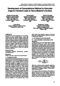
More information about these systems and other simulation environments can be found in Barber et al. (2007) [10]. In this paper we consider the random disturbances of knock-on delays and operation time. We introduce a microscopic simulation based method to analyze the carrying capacity of railway stations. We have developed a software platform to perform the analyzing process automatically. The paper is structured as follows. Section 2 shows the outline of the method. In Section 3, we introduce the switch grouping method. Section 4 presents the capacity analyzing method in detail. Section 5 provides a case study of Beijing South railway station. Finally, comes with the conclusion. Outline of the method Railway station capacity is tightly related with infrastructure of railway station, to analyze the capacity by computer program, the first step is modelling the infrastructure of railway station. Then divide all switches into different groups. The principles and methods will be introduced in detail in section 3. Due to complexity of railway system, there are always random disturbances during the daily operation, the theoretic capacity is only the reference capacity, usually cannot be reached. To analyze the realistic capacity of a railway station, we need consider random disturbances. Put many simulation results together, we can analyze the practicality capacity of the railway stations. The outline of the method is shown as Figure 1. Infrastructure Modelling Of railway station
Switch groups generation
Train operation plan re-scheduling
Switch groups occupation ratio calculation Random disturbance generation Calculate station capacity
Termination condition
N
Y Output and analyzing station capcacity
Figure 1:The outline of the method Automatic switch grouping method When a conflict occurs, one resource must be occupied by two operations at the same time. That means when a switch is occupied by an operation route, some other operations also apply using the same switch at the same time.
38
Figure 2:The example of switch groups If some switches are occupied by a train operation or shunting operation, the other switches in this switch group are not available. We put these unavailable switches and the occupied switches together into a group. This group is called “switch group”. The occupation time or exploitation rate of all switches which are in the same switch group is the same. For example, in Figure 2, if a train is occupying Route 1, switch 1 and switch 3 are occupied by the train. Meanwhile, the switch 5, 7, 9 are not available. Because Route 1 and any route which contains the switch 5 or 7 or 9 will be conflicting routes, such as Route 2, 3, 4. As the same reason, any one of switch 1, 3, 5, 7, 9 is occupied, the others are unavailable. Thus, the time or utilization of the switch 1, 3, 5, 7, 9 are the same. We consider switch 1, 3, 5, 7, 9 is in one “switch group”. If two switches are on two parallel routes respectively, the two switches shouldn’t be in the same switch group. If not, they should be in the same switch group. The microscopic simulation based method The exploitation rate method is a traditional method to calculate carrying capacity of railway stations. But the calculation results usually can’t truly reflect the capacity. Based on the traditional method of utilization and probability theory, we provide an analyzing method based on random probability. Train delays and operation time variation of route is considered in this section. The corresponding probability distribution is derived from large empirical data, and the disturbances is simulated by computer and put into the model. The calculation method of exploitation rate The basic idea of this method is to compute exploitation rate of each switch group in station based on current operation plan. Choose the most heavily used switch group, according to the existing number of trains and exploitation rate of switch, we can get the maximum number of trains during the whole service time span. The formulation of exploitation rate method is as follow. n
K =
∑
i =1
ti
(1)
T N=
n K
(2)
The variables used in exploitation rate method are defined as follows: T :The total operation time. Usually its value is 86400 seconds (24 hours). ti :The time of train i occupying the critical switch group K : Exploitation rate of the critical switch group n :The existing number of trains in each direction of a station N :Carrying capacity of throat for one direction of a station
39
According to exploitation rate method, first, we need to compute the exploitation rate of each switch based on equation (1). Finally, according to equation (2), we can obtain carrying capacity of throat in railway station. The arrival time and departure time distribution of trains It’s hard for all trains to arrive at the station on time. The arrival time of a train may fluctuate near the scheduled time. We adapt the Erlang distribution to model the arrival time distribution of a train (Yuan and Hansen, 2007) [7]. The probability density function of the Erlang distribution is as follows: f ( x; k , λ ) =
λ k xk −1e− λ x (∀x, λ ≥ 0) (k − 1)!
(3)
The parameter k is called the shape parameter, and the parameter λ is called the rate parameter. The cumulative distribution function of the Erlang distribution is as follows: k −1
1 −λx e (λ x ) n (∀x, λ ≥ 0) (4) n ! n= 0 For example, when k = 2, λ = 0.5 , the probability density function and cumulative distribution F ( x; k , λ ) = 1 − ∑
function are as follows: Figure 3(a) shows the distribution probability density curve and Figure 3(b) shows the cumulative Erlang probability distribution curve. 0.2
1
0.18
0.9
0.16
0.8
Cumulative probability
Probability density
0.14 0.12 0.1 0.08 0.06
0.7 0.6 0.5 0.4 0.3
0.04
0.2
0.02
0.1
0
0
2
4
6
8
10 t(min)
12
14
16
18
0
20
0
2
4
6
8
10 t(min)
12
14
16
18
20
(a) (b) Figure 3: The Erlang distribution curve of arrival time The extreme point is (2, 0.1839). When t = 2 , it means the train arrives on time. When t < 2 , it means the train arrives early. When t > 2 , it means the train arrives late. The train arriving disturbances will be generated according to this function. In a similar way, we use the Erlang distribution to model departure time distribution of a train. But the parameters are different. According to data analyzing results, we choose Erlang distribution with parameters of k = 2, λ = 2 . The cumulative distribution function is shown in figure 4.
40
1 0.9
Cumulative probability
0.8 0.7 0.6 0.5 0.4 0.3 0.2 0.1 0
0
0.5
1
1.5
2
2.5 t(min)
3
3.5
4
4.5
5
Figure 4: The Erlang distribution curve of departure time A train is not allowed to depart earlier than the scheduled departure time. So when t = 0 , it means the train departures on time. P ( t < 1.5) = 0.80 , P ( t < 2) = 0.90 , P ( t > 3) = 0.0005 . It means train departure disturbances range from 0 to 3 minutes. The operation time distribution of trains There is certain time standard for every train operation. However, in actual situation, the operation time may fluctuate. We use the normal distribution to model the operation time distribution of a train. The probability density of the normal distribution is: − 1 f ( x | µ,σ ) = e 2πσ
( x − µ )2 2σ 2
(∀x ≥ 0, σ > 0)
(5)
Here, µ is the mean or expectation of the distribution. In this paper it means the time standard of a certain operation. The parameter σ is its standard deviation. Here it means the size of the operation time fluctuation. To each operation, there is a provision that the actual operation time can’t less than 80% of the standard time. For example, if the standard operation time is 5 minutes. According to the provision the occupation time can’t less than 4 minutes. Case study We have developed a software platform to calculate carrying capacity of railway stations with the proposed simulation method. In this section we take Beijing South railway station as an example to calculate carrying capacity. The Beijing South Railway Station is one of the largest integrated transport terminals in China. There are receiving-departure yard, depot and temp yard in the station. The station is connected to four adjacent railway stations, a large depot, and has four yards: a regular-speed train yard, a high-speed train yard, an inter-city train yard and a temporary storage yard for inter-city trains. The station connects five directions, Liu Village, Beijing South turn, Depot, Lang fang and Yi Zhuang. (1) According to the existing data of Beijing South railway station, the system automatically calculates the theoretic carrying capacity of Beijing South railway station throat without considering the random disturbances. Table 1 shows the calculation results without disturbances.
41
Table 1: The theoretic capacity without disturbances (unit: trains/day) Direction
Arrival capacity
Departure capacity
Liu Village
351
339
Beijing South turn
215
224
Depot
151
103
Lang fang
332
332
Yi Zhuang Sum
560 1609
560 1558
(2) In this subsection we consider the random disturbances of train delay. When the probability of delay is from 0.7 to 0.95 and the delay time is from 60s to 210s, the first cell means 95% train will arrive at station within 60 seconds delay. We simulate 36 pair input parameters, and calculate the occupation rate to get total departure and arrival capacity (in Table 2) of Beijing South railway station. Table 2: Capacity with train delay disturbances (departure/arrival, unit: trains/day) Delay Time Probability 0.70 0.75 0.80 0.85 0.90 0.95
60s
90s
120s
150s
180s
210s
1598/1608 1628/1642 1634/1657 1579/1586 1677/1661 1655/1681
1571/1538 1518/1515 1533/1542 1545/1539 1587/1599 1625/1638
1391/1429 1454/1461 1510/1516 1413/1419 1548/1544 1609/1597
1387/1361 1357/1362 1410/1454 1332/1332 1525/1482 1491/1516
12481269 1293/1325 1349/1373 1286/1290 1469/1458 1509/1507
1264/1247 1208/1217 1269/1281 1196/1214 1367/1395 1420/1435
(3) In this section we consider random factor of operation time fluctuation. Calculation results are as follows. The first cell means 95% operations can be performed within 60 seconds. We simulate 36 pair input parameters, and calculate the occupation rate to get total departure and arrival capacity (in Table 3). Table 3: Capacity with operation time disturbances (departure/arrival, unit: trains/day) Delay time Probability 0.70 0.75 0.80 0.85 0.90 0.95
60s
90s
120s
150s
180s
210s
1399/1388 1429/1414 1438/1414 1381/1373 1445/1459 1460/1433
1332/1364 1321/1322 1340/1330 1336/1340 1392/1379 1420/1406
1252/1213 1273/1265 1314/1307 1223/1216 1346/1348 1385/1396
1179/1204 1179/1173 12681223 1167/1165 1287/1329 1315/1289
1108/1086 1156/1123 1188/1163 1129/1124 1270/1279 1309/1310
1082/1098 1055/1045 1117/1104 1056/1037 1217/1188 1250/1234
Comparing the calculation results of different methods, we can get the following conclusions. (1) The capacity with random disturbances is less than theoretic capacity. It is closer to the real ability of the station. (2) Less train delay disturbances can improve railway station capacity. What’s more, the greater the probability is, the greater the ability is. If 95% trains can arrive at station within 60 seconds, the total capacity is 1681. When 70% trains can arrive at station within 210 seconds, the total capacity is to 1247, and nearly 25.8% capacity decreases, as Table 5 shows. (3) Less operation time disturbances also can improve railway station capacity. Conclusions This paper provides a microscopic simulation method and a stochastic model for evaluating capacity of railway stations. The calculation results show that this computer aided tool can be used for general railway station capacity analyzing and is also beneficial to guiding design or expansion of
42
station. The models and method presented in this paper have been developed as application software which is running in several big railway stations in China. In further research, we will focus on: (1) Improving model and method of microscopic simulation based method. (2) The capacity we computed is about the carrying capacity of a railway station, and neglects other capacities such as line capacity, network capacity. How to integrate all these capacities and evaluate the railway network capacity is a more useful further research. Acknowledgments This work was financially supported by “the Fundamental Research Funds for the Central Universities (No. 2014JBZ008)” and Fundamental Research Funds of Beijing Jiaotong University (2011JBM065). References [1]
[2] [3] [4]
[5] [6] [7] [8]
[9] [10]
Abril, M., Salido, M.A., Barber, F., Ingolotti, L., Lova, A., Tormos, P. "A heuristic technique for the capacity assessment of periodic trains". Frontiers in Artificial Intelligence and Applications 131, 339–346, 2005. Burdett, R.L., Kozan, E. "Techniques for absolute capacity determination in railways". Transportation Research Part B 40, 616–632, 2006. Yungui Yang, Ciguang Wang, "The bayesian interval notation of station capacity". Statistics and decision, 165-167, 2011 Malavasi G, Molková T, Ricci S, et al. “A synthetic approach to the evaluation of the carrying capacity of complex railway nodes”[J]. Journal of Rail Transport Planning & Management, 2014, 4(1): 28-42. Caprara, A., Fischetti, M., Toth, P. "Modeling and Solving the Train Timetabling Problem", Research Report OR/00/9 DEIS, 2000. R. Ahuja, M. Jaradat, K. Jha, A. Kumar. "An Optimization-Based Decision Support System for Train Scheduling", White Paper, Innovative Scheduling, USA, 2006. Jianxin Yuan, Ingo A. Hansen. "Optimizing capacity utilization of stations by estimating knockon train delays". Transportation Research Part B 41, 202-217, 2007. Radtke, A., Hauptmann, D, "Automated planning of timetables in large railway networks using a microscopic data basis and railway simulation techniques". In: Allan, J. et al. (Eds.), Computers in Railways IX. WIT Press, Southampton, pp. 615–625, 2004 A. Nash, D. Huerlimann, "Railroad Simulation Using OpenTrack", Comprail, Dresden, Germany, 2004. Barber, F., Abril, M., Salido, M.A., Ingolotti, L., Tormos, P., Lova. A. "Survey of automated Systems for Railway Management", Technical Report DSIC-II/01/07, Department of Computer Systems and Computation, Technical University of Valencia, 2007.
43