a mixed integer linear programming approach to the optimal ... - PSCC

A MIXED INTEGER LINEAR PROGRAMMING APPROACH TO THE OPTIMAL CONFIGURATION OF ELECTRICAL DISTRIBUTION NETWORKS WITH EMBEDDED GENERATORS A. Borghetti, M. Paolone, C.A. Nucci Electrical Power Systems Laboratory - LISEP University of Bologna, Italy {alberto.borghetti;mario.paolone;carloalberto.nucci}@unibo.it Abstract – The paper focuses on the solution of the minimum loss reconfiguration problem of distribution networks, including embedded generation, by means of a mixed integer linear programming (MILP) model. The proposed model takes into account typical operating constraints of distribution networks (radial configuration, branch ampacity limits and bus voltage requirements). The accuracy of the results and the computational performances of the proposed MILP model are evaluated by making reference to test networks already adopted in the literature for the problem of interest.

Keywords: network reconfiguration, power loss minimization, radial networks, distribution systems, mixed integer linear programming, graph theory. 1 INTRODUCTION The choice of the configuration of a given electrical network that minimizes the losses and meets all the operating requirements is a typical problem for distribution system operators and has been successfully addressed by using various approaches. Recent reviews and classifications can be found in [1,2]. In particular, heuristic algorithms that start from a feasible network configuration have been proven to achieve good results in short runtimes [3]. The increasing installation of embedded generation, which frequently uses renewable, but fluctuating, energy resources, renovates the interest for the solution of the optimal configuration problem, also without the need to start from an initial feasible configuration. Recently, the efficiency of Mixed Integer Linear Programming (MILP) solvers have been significantly increased mainly by the adoption of cutting-plane capabilities [4], local search techniques (e.g. [5]), and effective heuristics techniques applied to the finding of a first feasible solution (e.g. [6]). A MILP model is defined by a linear objective function of the variables to optimize, some of which assume integer values, and a set of linear (equality or inequality) constraints. The optimal configuration problem of a distribution network is characterized by several nonlinearities, mainly represented by the power flow equations. The main issue in the application of MILP solvers is the efficient linearization of these equations. The following linearization approaches have been presented in the literature. In [7] an iterative procedure is applied to a single-loop linear problem, in which the

17th Power Systems Computation Conference

network loads are assumed as constant current injections and voltage drops in the lines are neglected. In [8] the linear d.c. power flow approximation is adopted. In [9] a genetic algorithm approach is compared with a MILP model in which the quadratic functions that represent the power flow in the lines are approximated by using piecewise linear functions (PLFs). Moreover, [2] presents a mixed-integer quadratically constrained problem, formulated so that non-linear multiplications between line statuses (represented binary variables) and continuous variables are avoided. This paper describes a MILP model of the reconfiguration problem that directly incorporates the typical operating constrains of distribution networks, namely radial configuration, branch ampacity limits and limited bus voltage deviations with respect to the reference value, taking into account the presence of embedded generation. To the best of the authors’ knowledge, some characteristics of the proposed MILP model, such as the linear representation of loads and embedded generation, have not been already dealt with in the literature on the subject. The approach is tested by using the reference networks analyzed in [2]. The structure of the paper is the following. Section II is devoted to the statement of the problem. Section III presents the MILP model. Section IV shows the numerical results obtained for various test networks of different size. Section V is devoted to the Conclusions. 2 THE PROBLEM The typical minimum losses configuration problem is defined as the search of the radial network configuration that corresponds to the minimization of the network losses. The configuration should permit to feed all the loads and to allow the production of all the embedded generators, with current flows below the ampacity limits of cables and overhead lines and bus voltage deviations lower than a predefined level of few percent with respect to the rated value. Furthermore, various multi-objective reconfiguration problems have been formulated and addressed in the literature. In these problems, other than the minimization of the losses, the objective function may include the minimization of voltage deviations (e.g. [10,11]) and of other power quality indices (e.g. [12]), the minimization of switching number (e.g. [10,13]), transformer load

Stockholm Sweden - August 22-26, 2011

balancing (e.g. [10,11]), the optimal placement of capacitor banks (e.g. [14]). This paper will focus on the solution of the minimum losses configuration problem. The electric power distribution network of N buses and Nb lines is associated to a connected graph G: each bus k being represented by one distinct element of the set K of the vertices of G and each line b being represented by one distinct element of the set B of edges of G. The point of connection of each load is a bus of the network and each couple of connected busses defines a different line. The considered networks do not have parallel edges and self-loops. A configuration of the network that does not contain closed paths (cycles) and that allows to feed all the loads is associated to a spanning tree of G. Each configuration of the network is represented by binary column vector u with Nb elements: ub=1 indicates that line b is connected, ub=0 indicates that the line is disconnected at both ends. The optimization model for the computation of the minimum loss configuration u* is written as follows: Nb

u*  arg min  Ploss,b

(1)

b 1

subject to

(2) xF * (3) u U where Ploss,b are the active power losses on line b, x is the set of phasors that represent the bus voltages and the line currents, U indicates the set of configurations each corresponding to a spanning tree of G and F the feasible operating region of the network. Objective function (1) minimizes the total value of line losses. Constraints (2) represent all the operating constraints that bound the bus voltage deviations below to a small percentage of rated value Vr and limit each line current below the relevant capability. Moreover, constraints (2) also include the network equations that also incorporate the characteristics of loads and embedded generators. Constraint (3) ensures that the network is radially operated. In order to obtain a MILP model, both the objective function and all the constraints of problem (1)-(3) must be expressed by linear relationships, involving binary decision variables u* and the associated vector x of continuous variables that describe the network operating conditions. 3 THE MILP MODEL We here assume to have the capability to change the status (connected or non-connected) of every line in the network. Moreover, for sake of simplicity in the model description, the amplitude of the voltage Vs at slack bus s is assumed equal to the rated value Vr. Vs is the reference for the phases of all the other voltages and the currents of the network. In the following sub-sections, the various parts of the proposed MILP model of problem (1)-(3) are presented:


the radiality constraint, the network equations, the line current bounds and the objective function and, finally, the constraints on the bus voltage deviations with respect to the rated value. 3.1 Radiality constraint The MILP radial configuration constraints ensure the opening of all the cycles of the graph associated to the distribution network. All the cycles can be efficiency determined by using a search strategy (e.g. [15]) or by the union of two or more cycles of a cycle basis [16]. The latter approach is here described. A spanning tree of G is readily obtained by a applying a depth-first search (DFS). Each of the Nb-(N-1) fundamental cycles associated to the spanning tree is defined by adding just one edge and by removing all the leaf nodes. As the set of the fundamental cycles associated to any of the spanning tree of G form a basis for the cycle space, all the simple cycles (i.e., without repeated vertices) are found by the union of two or more cycles of the basis. The union between two cycles is performed by applying the exclusive OR logic operation to the corresponding elements of the relevant u binary vectors. The implemented procedure inspects, again by a DFS, the union of each combination of two or more fundamental cycles in order to check whether it is a simple cycle and, in that case, adds the relevant u vector as a column of matrix L, the columns of which finally represents all the distinct Nc cycles in the graph. Constraint (3) is then represented by the following set of integer linear constraints Nb

 b 1

being

b, j

Nb

* b , j  ub   b 1

b, j

 1 j  1... N c

(4)

the b,j binary element of matrix L.

3.2 Network equations The network equations define the equilibrium of the currents at each bus and the voltage drops in each connected line. 3.2.1 Bus equations The equations include the models of loads and embedded generators. These equations are expressed as linear constraints by setting, at first, the real and imaginary parts of each phasors Ink, representing the current injected into bus k, as corresponding to the active power and reactive power relevant to the load or generator connected at bus k, assuming Vk=Vs. As the typical amplitude and phase deviations of Vk from Vs limited, we then apply the small variation approximation in order to find each correction Ink to be added to Ink so to represent the characteristics of load or generator injections at bus k. Assuming a symmetrical system operating condition, each line b is represented the usual one-phase Π equivalent circuit, each characterized by the values of resistance Rb, reactance Xb and total shunt capacitance 2Cb. Therefore, for each line each line b connected to


Even when the functions that describe Inkre and

bus k, the bus equations includes both current I b flowing in Rb, and Xb and current I bsh,k in Cb at bus k 1. For each bus, the two linear equality constraints relevant to the real part (superscript re) and imaginary part (superscript im) are the following:  I bre   I bsh,k,re  Inkre  Inkre k  K , k  s (5) bBk

I

bBk

bBk

im b

  I bsh,k,im  Inkim  Inkim k  K , k  s

(6)

bBk

where Bk is the set of lines b connected to bus k. The components Inkre and Inkim are functions of the deviations of the real and imaginary parts of Vk with respect to Vs, taking into account the following three cases. a) Loads represented by a constant injection Ink with fixed amplitude Ink and phase  k with

Inkim are linear, as in case a) and b), we have found more convenient, from the computational point of view, the implementation of a two-iterations procedure. In the first iteration, Inkre and Inkim are null, while in the

second, both are calculated by using the values Vkre and Vkim obtained in the first iteration.

3.2.2 Line equations The equations of the differences between the real and imaginary parts of the voltage phasors at the terminals h and k of each line b are represented by the following linear constraints: Vhre  Vkre  Rb  I bre  X b  I bim  vbre  0 b  B (13) vbre  BN  ub*  BN vbre  BN  ub*  BN

respect to the voltage phasor of the relevant bus k: 2 Vkim Vs

(7)

Vkim Vs

(8)

Inkre   Ink sin( k )  Inkim  Ink cos( k ) 

b) Loads and embedded generators represented by constant active P and reactive Q power injections (PQ nodes): 3 Inkre   Inkre  Inkim  Inkre 

c)

Vkre  Vs V im  Inkim  k Vs Vs

V V  Vs  Inkim  Vs Vs im k

re k

(9) (10)

Embedded generators represented by constant active power P injections with the capability to maintain the voltage amplitude equal to a set value Vk (PV node): constraints (5),(6),(9) and (10) are applied with Inkim as a continuous variable and the two following constraints are added 

Qmax,k 3Vs

 Inkim  

V

Qmin,k

(11)

3Vs

V

(12) In (11) the sign convention of positive powers and current components when injected in the bus from outside applies. Inkim permits to adapt the reactive power production taking into account the generator upper and lower limits. Constraint (12) is explained in sub-section 3.4. re 2 k

V

1

im 2 k

2 k

The inclusion of I b , k appears to be useful for the calculation of sh

the voltage amplitudes when the network is characterized by a large presence of cable lines. 2 If the angular deviation of Vk with respect to Vs is small, then the im ratio Vk Vs could be assumed as its approximation. 3 A null variation of the active power value implies

V

k

re



v  BN  u  BN im b

* b

vbim  BN  ub*  BN

(15) (16)

where BN is a big number, in this case, larger than the maximum voltage difference between unconnected busses 4. Constraints (14) and (16) ensure that auxiliary variables vbre and vbim are null when line b is connected. Alike, the real and imaginary parts of current I bsh,k of each line connected to bus k are represented by the following constraints: I bsh,k,re Cb  Vkim  vbre,k  0 vbre,k  BN  ub*  BN b  Bk , k  K , k  s (17) vbre,k  BN  ub*  BN I bsh,k,im Cb  Vkre  vbim,k  0 vbim,k  BN  ub*  BN b  Bk , k  K , k  s (18) im * vb,k  BN  ub  BN

being ω the rated value of the angular frequency. Auxiliary variables vbre,k and vbim,k are null when line b is connected and equal to - Vkim , respectively, and Vkre when disconnected (being I bsh,k,re and I bsh,k,im null). 3.3 Objective function and line current constraints Both the objective function and the maximum line constraint require the evaluation of the square value of the real and imaginary part of the line current phasors, defined by the network equations. For this purpose, a PLF approximation is adopted. Different PLF techniques, compared in [17], use binary variables or special ordered sets of variables (SOS2 [18]). For the PLF representation of the objective function and the line current constraints, the three following simplifying conditions apply: 1) the function to be represented is quadratic;

 Vs  Ink  Ink  Vs  Vk  Ink  0 re

re

im

im

and a null variation of the reactive power value implies Vk  Ink im

Vhim  Vkim  X b  I bre  Rb  I bim  vbim  0 b  B

(14)

re

 V  V   In  In re

k

s

im

im

k

k

 Vs  0 .


4

As explained in subsection 3.3, when line b is disconnected both im I b and I b are null. re


2) the minimum value of the currents is sought by the optimization problem; 3) the constraints are represented by upper bunds. These simplifying conditions permit to represent both the objective function and the line current constraints by means of the two following sets of linear constraints: - the first set permits the evaluation of I bre and I

b  B , which also ensure that current I b

im b

is null if line b is not connected (i.e., if ub* =0),

3.4 Bus voltage constraints For the bus voltages, simplifying conditions 2) and 3) do not apply. Therefore, in order to enforce the lower and upper boundaries to the bus voltage amplitude, we have included two additional binary variables, namely wkre,i and wkim,i for each interval i of the PLF model of the square value of Vk. The two sets of constraints representing the relevant PLF models are: - evaluation of Vkre and Vkim k  K , k  s Vkre  Vkre  0

I bre  I bre  0 I  I re b

I I

re b

im b

I

Vkim  Vkim  0

 I b,max  ub*  0 I

im b

im b

I

(20)

0

I bim  I b,max  ub*  0

and I bsh,k,re ) whilst the second set of constraints applies the PLFs to estimate the square values of the real part ( I bre 2 ) and imaginary part ( I bim 2 ) of each line current, (21)  I bre 2  bre,i  I bre   bre,i i  Zbre , b  B I

im 2 b

  I im b,i

im b

 

(22)

i  Z , b  B

im b,i

im b

where Z  {1... z } and Z  {1... z } are the set of breakpoints of the PLFs, and bre,i  I bre,i 1  I bre,i (23) i  1. .. zbre  1  bre,i  I bre,i 2  bre,i  I bre,i re b

re b

bim,i  I bim,i 1  I bim,i im 2 im im  im b ,i  I b ,i  b ,i  I b ,i

im b

im b

i  1. .. z  1 im b

(24)

being ( I bre,i , I bre,i 2 ) and ( I bim,i , I bim,i 2 ) the coordinates of each breakpoint i of the PLFs. Due to simplifying condition 1, equations (23) and (24) represent the slope and the ordinate intercepts relevant to each interval of the PLFs. Simplifying conditions 2 and 3 permit to avoid additional binary variables. Being I b2  I bre 2  I bim 2 , objective function (1) becomes Nb

R I b 1

re 2 b b

-

PLF models of the real and imaginary parts of Vk k  K , k  s , each specified by a set of breakpoints Zkre  {1... zkre } or Zkim  {1... zkim } ,

(analogous equations are written also for I bsh,k,re -

(28)

Vkim  Vkim  0

0

im b

(27)

Vkre  Vkre  0

(19)

0

re b

Nb

  Rb I bim 2

(25)

b 1

In the representation of the line ampacity constraints, we disregard the contribution of I bsh,k to the line current in order to reduce the number of the required PLF models: (26) I bre 2  I bim 2  I b2,max b  B

Vkre 2 

zkre 1

zkre 1

i 1

i 1

 kre,i  vkre,i 

zkre 1

 vkre,i  i 1

zkre 1

w

re k ,i

i 1

zkre 1

V

re k ,i

i 1

V

re 2 k ,i

 wkre,i  0

 wkre,i  Vkre  0

(29)

1

vkre,i  Vk ,max  wkre,i  0 i  1. .. zkre  1 Vkim 2  zkre 1

v i 1

im k ,i

zkre 1

w i 1

im k ,i

zkre 1

 kim,i  vkim,i  i 1



zkre 1

V i 1

im k ,i

zkre 1

V i 1

im 2 k ,i

 wkim,i  0

 wkim,i  Vkim  0

(30)

1

vkim,i  Vk ,max  wkim,i  0 i  1. .. zkim  1

where, kre,i  Vkre,i 1  Vkre,i i  1. .. zkre  1

(31)

kim,i  Vkim,i 1  Vkim,i i  1. .. zkim  1

(32)

In (29) and (30), additional continuous variables vkre,i and vkim,i represents the difference between the values of Vkre,i and Vkim,i with respect to the immediately preced-

ing abscissa of a PLF breakpoint. The third and fourth constraints in (29) and (30) guarantee that Vkre 2 and Vkim 2 are defined by only one of the intervals of the relevant PLF representations. Being Vk2  Vkre 2  Vkim 2 , the upper and lower bounds Vk,max and Vk,min of Vk become Vkre 2  Vkim 2  Vk2,max Vkre 2  Vkim 2  Vk2,min

k  K

(33)

being I b,max the maximum current amplitude value for each line b.



4 TEST RESULTS The model described in the previous section has been tested by using the CPLEX V12.2 MIP solver under Matlab R2009b on a 1.3 GHz Intel Quad Core processor with 4 GB of RAM, running 32-bit Windows. The tests have been carried out for the distribution networks analyzed in [2], which presents a detailed comparison of the results reported in the literature: the 15-bus 16-line system originally described in [19], the 32-bus 37-line system originally described in [20] and the 69-bus 74-line system firstly adopted in [21] as an enlargement of the radial network described in [22]. Moreover, [2] also presents the results for a 5-bus 7-line system in order to illustrate the effects of operating conditions and constraints not usually included, such as the presence of a PV node, the maximum current constraint in a line and the minimum voltage bounds. All the lines of the considered networks are assumed to be equipped with reconfiguration switches. Both the computational time and the accuracy depend on the number of intervals adopted for the PLF representation of the quadratic functions. In all the tests, the results have been obtained with the following number of intervals for the PLF models: for I b 2 , zbre = zbim =31 b  B

The comparison between the final MILP solution and the PF results corresponding to the minimum-losses configuration is summarized in Tab. 1. The table reports also the computer total time relevant to the Cplex solution of the two iterations. A slightly lower value of the network losses has been obtained by the MILP model due to the approximations associated to the use of (9) and (10) for the PQ-node representation.

a)

b)

for Vk 2 , zkre = zkim =4 k  K A maximum phase deviation with respect to the slack bus of 5°, i.e. the break points relevant to V are re 2

k

allocated between Vk ,min cos( / 36) and Vk ,max , whilst those relevant to Vkim 2 are allocated between 0 and Vk ,max sin( / 36) .

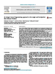
For each network, the minimum losses configuration obtained by using the proposed MILP model is compared with the results reported in the literature. Moreover, in order to assess the effects of the linear approximations, each MILP solution is also compared with the power flow (PF) results corresponding to the obtained optimal network configuration5. 4.1 5-bus 7 line system The slack bus has constant voltage equal to Vs=20 kV. At the end of line 3 is connected a an embedded generator G represented as a PV node with P=5 MW and V=0.97 p.u.. All the other 4 buses are represented by PQ nodes with the values reported in [2]. The network contains 3 distinct simple cycles. The three different tests presented in [2] are repeated here by using the proposed MILP model: namely the base test, the voltage test and the current test. 4.1.1 Base test In the base test the voltage and current operating constraints are not binding, i.e. Vk,max=1.1 p.u., Vk,min=0.9 p.u., and Ib,max=600 A. The minimum-losses radial configuration is shown in Fig. 1a) in which the two open lines are: 4 and 6. 5

c)

Figure 1 Optimal configurations of the 5-bus system: a) base test, b) voltage test, c) current test. The numbers indicate the lines according to the order of table B.1 of [2], whilst dotted lines indicate those open.

Losses (kW) Min. bus voltage (p.u.) (at the end of line no.) Max line current (A) (line no.) Load active power (MW) Load reactive power (Mvar) Active power injected by G (MW) Reactive power injected by G (Mvar) Slack bus active power (MW) Slack bus reactive power (Mvar) Cplex time (s)

PF reference results 637.658 0.9681 (1) 496.55 (7) 17.500 0.630 5.000 -10.260 13.138 11.103

MILP solution 632.204 0.9683 (1) 495.11 (7) 17.484 0.600 4.950 - 10.179 13.165 10.990 0.23+0.45

Table 1: Comparison between the MILP solution and PF results for the base test of the 5-bus system.

4.1.2 Voltage test In the voltage test the lower bound Vk,min = 0.97 p.u. has been imposed at every load bus. The minimumlosses radial configuration is shown in Fig. 1b) in which the two open lines are: 3 and 6. The comparison between the final MILP solution and the PF results corresponding to the minimum-losses configuration is summarized in Tab. 2.

The EMTP-rv load flow code [23] have been used.



Losses (kW) Min. bus voltage (p.u.) Max line current (A) (line no.) Load active power (MW) Load reactive power (Mvar) Active power injected by G (MW) Reactive power injected by G (Mvar) Slack bus active power (MW) Slack bus reactive power (Mvar) Cplex time (s)

PF reference results 647.114 0.970 (at G) 497.40 (1) 17.500 0.630 5.000 -10.270 13.147 11.137

MILP solution 644.529 0.970 (at G) 496.64 (1) 17.492 0.589 4.968 - 10.248 13.168 11.071 0.23+0.36

Table 2: Comparison between the MILP solution and PF results for the voltage test of the 5-bus system.

4.1.3 Current test In the current test Ib,max=368.9A has been enforced at line 5. The minimum-losses radial configuration is shown in Fig. 1c) in which the two open lines are: 4 and 7. The comparison between the final MILP solution and the PF results corresponding to the minimum-losses configuration is summarized in Tab. 3.

Losses (kW) Min. bus voltage (p.u.) (at the end of line no.) Max line current (p.u.) (line no.) Load active power (MW) Load reactive power (Mvar) Active power injected by G (MW) Reactive power injected by G (Mvar) Slack bus active power (MW) Slack bus reactive power (Mvar) Cplex time (s)

PF reference results 855.206 0.9455 (5) 551.64 (6) 17.500 0.630 5.000 -12.660 13.355 13.668

MILP solution 859.356 0. 9461 (5) 554.60 (6) 17.449 0.579 4.965 - 12.860 13.343 13.818 0.25+0.14

The comparison between the final MILP solution and the PF results corresponding to the minimum-losses configuration is summarized in Tab. 4. the results are in agreement with those presented in the literature [2].

Losses (kW) Min. bus voltage (p.u.) (at the end of line no.) Max line current (A) (line no.) Load active power (MW) Load reactive power (Mvar) Slack bus active power (MW) Slack bus reactive power (Mvar) Cplex time (s)

PF reference results 466.127 0.9716 (20) 355.76 (16) 28.700 5.900 29.166 6.445

MILP solution 465.971 0.9719 (20) 355.25 (16) 28.680 5.877 29.145 6.421 0.55+0.36

Table 4: Comparison between the MILP solution and LF results for the 15-bus system.

4.3 32-bus 37-line system The slack bus has constant voltage equal to Vs=12.66 kV, all the other 32 buses are represented by PQ nodes. The network contains 26 distinct simple cycles. The minimum loss configuration obtained without any voltage and current binding constraint (i.e. Vk,max=1.1pu. Vk,min=0.9p.u., Ib,max=300A) is shown in Fig. 3, in which the 5 open lines are: 7, 9, 14, 32, and 37. The comparison between the final MILP solutions and the PF results corresponding to the minimum-losses configuration is summarized in Tab. 5. The obtained results are in agreement with those presented in the literature [2].

Table 3: Comparison between the MILP solution and PF results for the current test of the 5-bus system.

The obtained results are in agreement with those presented in [2]. 4.2 15-bus 16-line system The slack bus has constant voltage equal to Vs=23 kV, all the other 15 buses are represented by PQ nodes. The network contains 7 distinct simple cycles. The minimum loss configuration obtained without any voltage and current binding constraint (i.e. Vk,max=1.1 pu. Vk,min=0.9 p.u., Ib,max= 400 A) is shown in Fig. 2, in which the 3 open lines are: 17, 19, 26.

Figure 3 Optimal configuration of the 32-bus system. The numbers indicate the lines following the order of [20], whilst dotted lines indicate those open.


PF reference results 139.552 0.9378 (31) 207.13 (1) 3.715 2.300 3.855 2.402

MILP solution 140.799 0.9388 (31) 206.52 (1) 3.704 2.292 3.842 2.393 9.06+7.50

Table 5: Comparison between the MILP solution and PF results for the 32-bus system.

Figure 2 Optimal configuration of the 15-bus system. The numbers indicate the lines according to Fig. 2 of [19], whilst dotted lines indicate those open.


4.4 69-bus 74-line system The slack bus has constant voltage equal to Vs= 12.66 / 3 kV, all the other 69 buses are represented by PQ nodes. In [21], three load conditions are examined, indicated as normally loaded system, heavyloaded system (multiplying each load demand by 1.2) and a light-loaded system (multiplying each load de-


mand by 0.5). The network contains 24 distinct simple cycles. For all the three load conditions, the minimum-losses radial configuration obtained without any voltage and current binding constraint (i.e. Vk,max=1.1pu. Vk,min=0.9p.u., Ib,max=200A) is shown in Fig. 4, in which the five open lines are: 15, 59, 62, 70, and 71 6.


PF reference results 7.177 0.9734 (61) 57.16 (1 and 2) 0.554 0.449 0.561 0.457

MILP solution 7.915 0.9737 (61) 57.32 (1 and 2) 0.554 0.449 0.561 0.457 27.41+20.19

Table 8: Comparison between the MILP solution and PF results for the 69-bus system lightly loaded. Figure 4 Optimal configuration of the 69-bus system. The numbers indicate the lines following the order of [21], whilst dotted lines indicate those open.

The configuration of Fig. 4 is the same as the one obtained in [2] for the normal case, whilst differs from the one obtained in [2] both for the heavy case (lines 15 and 61 are open instead of lines 13 and 64 as in [2]), and for the light case (lines 70 and 62 are open instead of lines 13 and 64 as in [2]). The network losses calculated by using the PF code for the heavy-case configuration of [2] are equal to 44.770 kW, whilst for the light-case configuration of [2] are equal to 7.674 kW. Both values are larger than the losses corresponding to the configuration of Fig. 4. The comparison between the final MILP solutions and the PF results corresponding to the minimum-losses configuration is summarized in Tab. 6, Tab. 7 and Tab. 8, for the normally, heavily and lightly loaded cases, respectively.


PF reference results 30.093 0.9452 (61) 116.14 (1-and 2) 1.108 0.898 1.138 0.931

MILP solution 30.554 0.9461 (61) 115.88 (1-and 2) 1.106 0.895 1.135 0.928 31.09+17.86

5 CONCLUSIONS The paper has addressed the problem of determining the minimum loss radial configuration of a distribution network. The proposed MILP model takes into account the main operating constraints other than radiality, such as the lower and upper bounds of the bus voltages and the upper limits of the line currents. As the network equations are written in terms of relationships between voltages and currents, the model incorporates also the line shunt capacitances useful for an accurate estimation of bus voltages in cable networks. The solution of the MILP model does not require the knowledge of an initial feasible configuration of the network. The results of the tests carried out on the four systems analyzed by Romero-Ramos et al. in [2] demonstrate the good accuracy of the proposed MILP model The reasonable accuracy on the evaluation of the final losses has been verified by its comparison with the LF results corresponding to the obtained optimal network configurations. Also the computational times appear reasonable. AKNOWLEDGEMENTS The IBM ILOG CPLEX Optimization Studio Version: 12.2 has been made available to the Authors laboratory through the IBM Academic Initiative. REFERENCES [1]

Table 6: Comparison between the MILP solution and PF results for the 69-bus system normally loaded.


PF reference results 44.210 0.9335 (61)

MILP solution

[2]

44.512 0.9348 (61) [3]

140.30 (1 and 2) 1.329 1.078 1.374 1.126

139.83 (1 and 2) 1.325 1.073 1.369 1.121 30.90+23.41

Table 7: Comparison between the MILP solution and PF results for the 69-bus system heavily loaded. 6

Note that opening one of the three lines 56, 57, 58 or 59 is indifferent as the loads at the end of the three lines 56, 57 and 58 are null.


[4]

[5]

R. F. Sarfi, M. M. A. Salama, and A. Y. Chikhani, “A survey of the state of the art in distribution system reconfiguration for system loss reduction”, Electric Power Systems Research, vol. 31, pp. 61–70, 1994. E. Romero-Ramos, J. Riquelme-Santos, J. Reyes, “A simpler and exact mathematical model for the computation of the minimal power losses tree”, Electric Power Systems Research, vol. 80, pp. 562–571, 2010. C. Ababei, R. Kavasseri, “Efficient network reconfiguration using minimum cost maximum flow based branch exchanges and random walks based loss estimations”, IEEE Trans. on Power Systems, Vol. 26, No. 1, pp. 30-37, 2011. R.E. Bixby, M. Fenelon, Z. Gu, E. Rothberg, R. Wunderling, “MIP: theory and practice – closing the gap”, in: System modeling and optimization: Methods, theory, and applications, Kluwer Academic Publishers, Dordrecht, pp. 19–49, 2000. E. Danna, E. Rothberg, C. Le Paper, “Exploring relaxation induced neighborhoods to improve MIP solutions”, Mathematical Programming, vol. 102, pp. 71–90, 2005.


[6] [7]

[8]

[9]

[10]

[11]

[12]

[13]

[14]

[15] [16] [17]

[18]

[19]

[20]

[21]

[22]

[23]

M. Fischetti, F. Glover, A. Lodi, “The Feasibility Pump”, Mathematical Programming, vol. 104, pp. 91-104, 2005. J.-Y. Fan, L. Zhang, J.D. McDonald, “Distribution Network Reconfiguration: Single Loop Optimization”, IEEE Trans. on Power Systems, Vol. 11, No. 3, August 1996. A. Abur, “Determining the optimal radial network topology within the line flow constraints,” in Proc. IEEE Int. Symp. Circuits Syst., vol. 1, pp. 673–676, May 1996. E. Romero Ramos, A. Gómez Expósito, J. Riquelme Santos, F. Llorens Iborra, “Path-Based Distribution Network Modeling: Application to Reconfiguration for Loss Reduction”, IEEE Trans. on Power Systems, vol. 20, no. 2, May 2005. A. Augugliaro, L. Dusonchet, S. Favuzza, E. Riva Sanseverino, “Voltage Regulation and Power Losses Minimization in Automated Distribution Networks by an Evolutionary Multiobjective Approach”, IEEE Trans. on Power Systems, vol. 19, no. 3, pp. 1516-1527, August 2004. A. Ahuja, S. Das, A. Pahwa, “An AIS-ACO Hybrid Approach for Multi-Objective Distribution System Reconfiguration”, IEEE Trans. on Power Systems, vol. 22, no. 3, pp. 1101-1111, August 2007. J. C. Cebrian, N. Kagan, “Reconfiguration of distribution networks to minimize loss and disruption costs using genetic algorithms”, Electric Power Systems Research, vol. 80, pp. 53–62, 2010. N. Gupta, A. Swarnkar, K.R. Niazi, R.C. Bansal, “Multiobjective reconfiguration of distribution systems using adaptive genetic algorithm in fuzzy framework”, IET Generation, Transmission & Distribution, vol. 4, no. 12, pp. 1288-1298, 2010. M.A.N. Guimarães, C.A. Castro, R. Romero, “Distribution systems operation optimization through reconfiguration and capacitor allocation by a dedicated genetic algorithm”, IET Generation, Transmission & Distribution, vol. 4, no. 11, pp. 12131222, 2010. R. Tarjan, “Enumeration of the elementary circuits of a directed graph”. J. SIAM, vol. 2, pp. 211–216, 1973. R. Diestel, Graph Theory, Fourth Edition, Springer -Verlag, Heidelberg, Graduate Texts in Mathematics, Volume 173, 2010. A. Keha, I. de Farias, and G. Nemhauser, “Models for representing piecewise linear cost functions”, Operations Research Letters, vol. 32, pp. 44-48, 2004. E. M. L. Beale and J.A. Tomlin, “Special facilities in general mathematical programming system for non-convex problems using ordered sets of variables”, Proc. 5th IFORS Conference, pp. 447-454, 1970. S. Civanlar, J.J. Grainger, H. Yin, S.S.H. Lee, “Distribution feeder reconfiguration for loss reduction”, IEEE Trans. on Power Delivery, Vol. 3, No. 3, pp. 1217-1223, July 1988. M.E. Baran, F.F. Wu, “Network reconfiguration in distribution systems for loss reduction and load balancing”, IEEE Trans. on Power Delivery vol. 4, no. 2, pp. 1401–1407, April 1989. H.D. Chiang, R.M. Jean-Jumeau, “Optimal network reconfigurations in distribution systems, Part 2: solution algorithms and numerical results”, IEEE Trans. on Power Delivery, vol. 5, pp. 1568–1574, July 1990. M.E. Baran, F.F. Wu, Optimal capacitor placement on radial distribution systems, IEEE Trans. on Power Delivery, vol. 4, no. 1, pp. 725–734, January 1989. J. Mahseredjian, S. Dennetière, L. Dubé, B. Khodabakhchian, and L. Gérin-Lajoie, “On a new approach for the simulation of transients in power systems”, Electric Power System Research, vol. 77, no. 11, pp. 1514–1520, Sep. 2007.

17th Power Systems Computation Conference Powered by TCPDF (www.tcpdf.org)
