z0= 0 %pi/2 0 0] t=0:0.1:10 xx=ode(z0,0,t,pend) .... 1/2*m*((v 1]+p*sin(alpha)*phi d])^2+. (v o]-p*alpha ... expand(subs(phi d]=kappa*v 1],v o]=0,L)))),v o]):.
A mixed symbolic - numeric software environment S. L. Campbell�, F. Delebecquey and D. von Wissel y � Dept. of Mathematics, North Carolina State University, Raleigh NC 27695 - 8205 - USA y INRIA - Rocquencourt, 78153 Le Chesnay Cedex - France 1. Introduction The objective of this paper1 is to illustrate the use of a Maple to Scilab interface (Scilab is a free CACSD package developed at INRIA.
ftp://ftp.inria.fr/INRIA/Projects/Meta2/Scilab http://www-rocq.inria.fr/scilab
). We show that the interface is a powerful tool for analyzing nonlinear systems and illustrate the interface on examples of the modeling and control of mechanical multibody systems.
Many control applications require the use of both symbolic and numeric computation. An illustrative example is the analysis and controller design of a mechanical system. To begin with, we need to compute the equations of motion. To study local stability we need to compute its linearization. To apply control concepts like feedback linearization we may need to compute the inverse system. All these operations are symbolic computations. To continue, we may want to do a computer simulation of the nonlinear system, study stability of the linearization at di�erent operating points or try a nonlinear controller. These are numerical operations evaluating the symbolic objects obtained before. In the applications we have in mind, we rst use symbolic computation. Then we need to transfer symbolic objects to numerically evaluable objects and nally we work with these new objects in a numerical environment. The opposite direction, that is the transfer of a numerical objects into a symbolic object is often of no interest. Indeed symbolic calculations are essentially based on rational numbers i.e. each number is associated with a pair a two \bignums" representing its numerator and its denominator. This representation allows to perform e�ciently exact calculations [5, 4] involving e.g. polynomials and is well suited to study speci c problems which depend on a few number of parameters. For instance it is well suited for studying parametric controllability of a linear system. However it is di�cult to use this approach if the basic data are
oating point numbers. In that case, after conversion 1 Research
partially
9423705, ECS-9500589
supported
by
INT-9220802,
DMS-
to rational numbers, the symbolic algorithm is likely to return a generic result. For instance any oating point matrix converted to rational numbers will be considered as full rank by a symbolic package eventhough it has a arbitrarily small singular values. In other words, the use of symbolic package in that context may lead to non robust results. Our approach is based on the use of symbolic package for generating speci c numerical Fortran or C code which is dynamically linked to Scilab.
2. Software tools We use Maple for symbolic and Scilab for numerical computation. What we need is an interface that permits these tools to communicate with each other. One realization of this interface is to incorporate the Maple kernel in Scilab. This would allow one to perform symbolic operations within the Scilab environment. However, as a matter of fact, only a few Maple functions would be available since symbolic computation requires a di�erent data structure and available Maple operations have to be compatible with the existing Scilab data structure. Another realization of the desired interface is to keep Maple and Scilab separated and to handle the transfer by an external tool. The latter structure allows one to use the original software (thus keeping all of its advantages). There is no need to nd a compromise between two essentially incompatible data structures. Furthermore, this approach makes the transfer transparent to the user and allows the use of compiled code (Fortran or C) for the numerical evaluation of Maple objects. Since the applications we have in mind require the use of numerous Maple facilities and execution time for the numerical evaluation of the Maple objects is important (mechanical multibody systems often involve large expressions), we have opted for the latter approach for the interface considered here. The key point of this interface is the facility of dynamic linking available in Scilab. The interface is based on the Maple
expressions into Scilab functions. Using Macrofort2 , we transfer the Maple object into a Fortran (or C) subroutine and dynamically link the code to Scilab. The linked code can be called like any other Scilab function with constant matrix parameters. For the applications that we consider, such as simulation and control of large dynamic systems, it is important to generate code which can be compiled. For instance, for ode simulations we generate a standalone Fortran subroutine with a speci c calling sequence compatible with Scilab ode solvers. Another very important aspect is the use of Maple optimize facility which allows to nd common subexpressions in a symbolic matrix, thus producing e�cient code.
Maple
maple2scilab
Macrofort
Scilab Dynamic link
Fortran The syntax of the function maple2scilab is the following: maple2scilab(fname; maplematrix; parameters) maplematrix is the name of the Maple matrix to be transfered and admitting parameters as parameters (list of vectors or matrices). fname is the name of the gener-
ated Scilab function: this function returns the numerical value of the transfered matrix for given values of input parameters. A similar function exists for sparse matrices. maple2scilab generate two les: fname.f and fname.sci which contain Fortran and Scilab code. Compilation of the numerical code can be easily automatized by a short shell script, making the transfer transparent to the user.
3. Examples In this section we illustrate the approach on two examples.
3.1. Inverted pendulum
In this well known example, the state variables are the position of the cart x = q1 and the angle � = q2. Below 2 Macrofort and
MacroC are Maple libraries that can be found
in the Maple share-directory
L = m1 +2 m2 x_ 2 + �_ 2 (J=2 + l2 m22 =2) + lm2 cos(�)(x_ �_ ; g) L:=qd[1]^2*(m[1]+m[2])/2+qd[2]^2*(J/2+l^2*m[2]/2)+ qd[1]*qd[2]*l*m[2]*cos(q[2])-g*l*m[2]*cos(q[2]); q:=vector(2);qd:=vector(2);qdd:=vector(2);m:=vector(2); S1:=grad(L,qd); S2:=evalm(grad(L,q)jacobian(S1,q)&*qd-jacobian(S1,qd)&*qdd); F:=subs(qdd[1]=0,qdd[2]=0,evalm(S2)); M:=jacobian(S2,qdd); maple2scilab(`msci`,M,[q,l,m,g,J]); maple2scilab(`fsci`,F,[q,qd,l,m,g,J]);
This yields the equations of motion � � M �x = F where matrix M and vector F are directly available as Scilab functions msci and fsci which evaluate M and F as function of the input parameters q,l,m,g,J. maple2scilab generated: subroutine msci(q,l,m,g,J,fmat) implicit double precision (t) double precision q(2),l,m(2),g,J,fmat(2,2) t4 = l*m(2)*cos(q(2)) t5 = l**2 fmat(1,1) = -m(1)-m(2) fmat(1,2) = -t4 fmat(2,1) = -t4 fmat(2,2) = -J-t5*m(2)**2 end function var=msci(q,l,m,g,J) var=fort('msci',q,1,'d',l,2,'d',m,3,'d',... g,4,'d',J,5,'d','out',[2,2],6,'d')
A simulation of the pendulum for a given proportional control u is then easily obtained by the following Scilab script: link('fsci.o','fsci');getf('fsci.sci','c') link('msci.o','msci');getf('msci.sci','c') l=1;m=[1;.1]J=.1;g=9.81; deff('zd=pend(t,z)',.. 'q=z(1:2),qd=z(3:4);u=K*(z-zop);.. zd=[qd;inv(msci(q,l,m,g,J))*.. fsci(q,qd,l,m,g,J)+[u;0]]') z0=[0;%pi/2;0;0];t=0:0.1:10; xx=ode(z0,0,t,pend);
� ; g=p sin(�) = 1=p cos(�) (1) is obtained by assuming that we control � directly by the acceleration of the cart x.
3.2. Simpli ed bicycle model
In this section we consider a more complex constrained mechanical system (which has in addition nonholonomic constraints). In this case, it is much more di�cult to obtain the equations of the model. A blind application of the Euler Lagrange equations, introducing Lagrange multipliers for the nonholonmic constraints leads to a much more complex model in implicit form in which all variables are coupled. The main di�culty is to nd an appropriate change of coordinates for simplifying the equations of motion. This part requires many symbolic computations which cannot easily be automatically implemented. The model considered here is a simpli ed bicycle model introduced by N. Getz [6]. P
α
2
m
∆
∆ z p J
rw
_ we have for the is small against the steering velocity �, kinetic energy of the steering wheel 2 2 _ 2 � J �_ 2 = J l1 �_2 2 2 Tkin = J2 (�_ + �) 2 2 (1 + � l1 ) which yields for the Lagrangian: 2 2 ; � L = m2 x_ 22 + y_22 + z_22 + J2 (1 +l1��_2l2 )2 ; g m z2 (4) 1 where x_ 2; y_2 and z_2 are computed from (3). Let � denote the lean angle of the bicycle, set c� = cos(�) and s� = sin(�), and de ne the partitioned generalized coordinates and velocities of the bicycle as follows: r = (�1; �; �)T ; r_ = (�_ 1; �;_ �_ )T , r_ = (v1 ; �; _ �_ )T _ T , s_ = (v0; �) _T s = (�0; �)T ; s_ = (�_ 0 ; �) R
where �1 = 0t v1 dt is the arc length of the trajectory of the contact R point of the rear wheel in the xy plane and �0 = 0t v0 dt. In these velocity coordinates the nonholonomic constraints become �v1 = �,_ v0 = 0, or equivalently � � 0 0 0 s_ + A_r = 0; where A = ;� 0 0 (5)
0
P1
P3
x
y
l1 l
0
Figure 1 Simple bicycle model considered by Getz [6] We denote by x1; y1 (resp. x2; y2) the plane coordinates of P1 (resp. P2 ) and � = tan(�)=l1 . The xycoordinates of the velocity of P1 are � � � �� � x_ 1 = cos(�) ; sin(�) v1 (2) y_1 sin(�) cos(�) v0 where v0 is the velocity of P1 perpendicular to the contact line P1 P3, and v1 the velocity parallel to P1P3 (rolling direcion). The rolling without sliding condition is v0 = 0 and we have from (2) the nonholonomic constrains: x_ 1 = v1 cos(�); y_1 = v1 sin(�) To write the Lagrangian, we need the velocity of the point mass m at P2 = (x2 ; y2; z2 ). We have x2 = x1 + cos(�) l0 + sin(�) sin(�) p y2 = y1 + sin(�) l0 ; cos(�) sin(�) p (3) z2 = p cos(�)
The Lagrangian is computed from (4), substituting x_ 2; y_2 and z_2 by (3), and x_ 1 and y_1 by (2) As shown in [1, 6, 3], the equations of motion can be computed using a \constrained" Lagrangian Lc obtained by substituting the constraints into the Lagrangian. Lc (ri ; r_ i) = L(ri ; ;Aji (r)_rj ) where s_j + Aji (r)r_j = 0. We obtain where
c @Lc @L i l V := dtd @L @ r_j ; @rj + @ s_i Bj;l r_ = 0
(6)
i i i = @Aj ; @Al Bj;l @rl @rj which can be written in the following form: M(r)r = F(r; r_) where M(r) := @V=@r and F := V ; M(r)r.
For the bicycle model Lc is computed from L setting v0 = 0 and �_ = �v1 This yields the simple bicycle model, which is composed out of the dynamical part, containing the reduced order equations of motion, and
straints. Furthermore, we need to a vector of generalized forces G(r)u representing the control inputs. We take a steering torque and a pedalling torque as control inputs. Dynamical part f8M(r)r = F (r; r_) + G(r)u �_ = v1 � < (7) Kinematic part : x_ 1 = v1 cos(�) y_1 = v1 sin(�) Designing a controller for such a model is unnecessarily complex. On the contrary, using the above decoupled model a controller is easily designed. Maple program to compute the reduced equations of motion: We have implemented the procedure described
before as a Maple script. The key step in this procedure is the change of coordinates that puts the nonholonomic constraint in the special form (5). In particular it is not easy to determine the partitioning of the variables. There is no systematic procedure for executing this step. The remaining steps can easily be translated into a Maple script. To this end we use the following set of generalized coordinates foo � bar � � q1 q2 q3 q4 q5 v0 v1 �_ �_ �_ qd1 qd2 qd3 qd4 qd5 v_ 0 v_ 1 � � � qdd1 qdd2 qdd3 qdd4 qdd5 Below is the resulting Maple session (l1 = b; l0 = c). L:=-m*G*p*cos(alpha) + 1/2*J*(b*kappa[d]/(1+b^2*kappa^2))^2+ 1/2*m*((v[1]+p*sin(alpha)*phi[d])^2+ (v[o]-p*alpha[d]*cos(alpha)+c*phi[d])^2+ (p*alpha[d]*sin(alpha))^2);
�
Jb2 �d 2 2 + m=2 (v1 + p sin(�)�d )2 L = ;mgp cos(�) + 2 (1+ b2 �2 ) + (vo ; p�d cos(�) + c�d )2 + p2 �d2 (sin(�))2
c
4
4
5
r:=subs(sg,vector([foo,alpha,kappa])); rd:=subs(sg,vector([v[1],alpha[d],kappa[d]])); s:=subs(sg,vector([foo,phi])); sd:=subs(sg,vector([v[0],phi[d]])); A:=matrix(2,3,[0,0,0,-q[5],0,0]); V:=proc(al) d_dt(diff(L_c,rd[al]))-diff(L_c,r[al])+ sum('A[a,al]*diff(L_c,s[a])','a'=1..2)+ sum('sum('diff(L0,sd[b])*B(b,al,be)*rd[be]', 'be'=1..3)','b'=1..2); end; B:=proc(b,al,be) diff(A[b,al],r[be])-diff(A[b,be],r[al]); end; d_dt:=proc(f) #The function d_dt differentiates f(q) and replaces #the q' by dq, qd' by qdd respectively. eval(innerprod(grad(f,q),qd)+ innerprod(grad(f,qd),qdd));end; V1:=subs(m=1,vector(3,V)); M:=jacobian(convert(V1,vector), vector([qdd[3],qdd[4],qdd[5]]));
2 6
M := 64
M11 M12 0 M12 p2 0 0 0 M33
3 7 7 5
where M11 = 1 + 2 p sin(q4)q5 + p2 (sin(q4))2 q52 + c2 q52 M12 = ;p cos(q4)cq5 Jb2 M33 = (1 + b2 q52 )2 F:=convert(map(collect,map(expand, subs(qd[2]=q[5]*qd[3],qd[1]=0,qdd[1]=0,qdd[2]=0,qdd[3]=0, qdd[4]=0,qdd[5]=0,evalm(V1))),{qd[3],qd[4],qd[5]}),matrix);
q:=vector(5);qd:=vector(5);qdd:=vector(5); sg:=v[o]=qd[1],phi[d]=qd[2],v[1]=qd[3], alpha[d]=qd[4],kappa[d]=qd[5],foo=q[1], phi=q[2],bar=q[3],alpha=q[4],kappa=q[5]; L0:=subs(sg,L);#unconstrained lagrangian LG2:=collect( expand(subs(cos(alpha)^2=1-sin(alpha)^2, expand(subs(phi[d]=kappa*v[1],v[o]=0,L)))),v[o]): L_c:=subs(sg,LG2);#constrained lagrangian
5
+m=2]qd3 2 ; mpqd cos(q4)cq qd ; mgp cos(q4) ; 4 � 5 3 2 2 2 2 2 +Jb qd5 =(2 1 + b q5 ) + mp2 qd4 2 =2
2
F1 6 F := 64 F2 ; g p sin(q4 ) F3 F1 =
;;
�
3 7 7 5
2 p2 sin(q4 )q52 + 2 p q5 cos(q4 )qd4 + � � � c2 q5 + p sin(q4) + p2 (sin(q4))2 q5 qd5 qd3
F2 = F3
;
4
�
;p cos(q4 )q5 ; p2 sin(q4)q5 2 cos(q4) qd32 ;
p cos(q4)c qd3 qd5 2 4 2 b2qd5 2q5 5 q5 = ; 2 Jb qd = ; M 33 (1 + b2q5 2) (1 + b2q52 )3
For the vector of generalized forces we have 2
u2 =m G(r)u := 4 0 u1 =m
3 5
This bicycle model can be controlled using various control strategies. We can use system inversion for tracking the lean angle of the bicycle to a desired trajectory. This is possible because the bicycle is with this choice of output a minimum phase system [6]. First, we consider linear feedback control for stabilizing the bicycle dynamics. For this we need to compute the linearization of the bicycle model. This is easily done in Maple. The linearization is of the form @ (F(r; r_) ; M(r)r)�r + @ F (r; r_ )� r_ M(r)�r = @r @ r_ which needs to avaluated at r = rop , r_ = r_op and r = rop . In the case of the bicycle we can assume that rop = 0. To compute the linear system in rop it su�ces to compute the Jacobian of F with respect to (�; �; v1; �;_ �): _ ff_x:=jacobian(convert(F,vector), vector([q[4],q[5],qd[3],qd[4],qd[5]]));
The simulation function in Scilab are msci() and ff(). They are simular to those of the inverted pendulum and will not be reproduced here. For computing a linear feedback matrix K we proceed as follows: the linearization is given by x_ = Ax + Bu where x = (��; ��; �v1; � �;_ � �) _ T : The following scilab script computes A and B. F_x=[0 0 0 1 0; 0 0 0 0 1; ff_x(r_op,rd_op,par)]; E=[eye(5,2),[zeros(2,3);msci(q0,qd0,par)]]; iE=inv(E); A=iE*F_x; B=iE*[zeros(2,2);0 1;0 0;1 0]
In this paragraph we use system inversion ideas to nd a trajectory tracking controller for the lean angle. Considering the lean angle and the velocity as output the resulting system is minimum phase.
0.30 0.23 0.16 � 0.09 0.02 −0.05 � −0.12 −0.19 −0.26 −0.33 −0.40 0.0 0.9 1.8 2.7 3.6 4.5 5.4 6.3 7.2 8.1 9.0
Figure 2 Linear stabilizing control
11.0 9.8 8.6 7.4 6.2 5.0 3.8 2.6 1.4 0.2 Start −1.0 −6.0−4.3−2.6−0.9 0.8 2.5 4.2 5.9 7.6 9.3 11.0
Figure 3 The resulting trajectory in the xy-plane. The input transformation �
�
"
�
�
#
�
2 b2 � _ 2� u1 = M33 � + (1+ 1 b2 �2 ) m + w u2 w 2 (M11v_1 + M12� ; F1)m puts the model into the form
8 < : 8 < :
� v_ 1 p2 � ; g p sin(�) �_ x_ 1 y_1
= = = = = =
�
(8)
w1 w2 cos(�)�(�; �_ ; v1; w2; �) v1 � v1 cos(�) v1 sin(�)
(9) �(�; �_ ; v1; w2; �) = � w2 p l0 + (�2 p2 sin(�) + � p)v1 2+ v1 �_ p l0 (10) To compute a tracking controller for the output y = (�; v) using the system inversion approach we need to di�erentiat the output untill we have an expression which can explicitly be solved for w. Noting that � is decoupled, we may assume that � is controlled by v_ 1 and �_ . This simpli es considerably the design procedure. Roughly speaking this amounts considering � as
is similar to the simpli ed equations of motion of the pendulum (1). Here again, a blind application of system inversion is possible using Maple, but this lead to an unnecessarily complex expression for the controller. 0.15 0.12 0.09 0.06 0.03 0.00 −0.03 −0.06 −0.09 −0.12 −0.15
� �d
Figure 6 The resulting trajectory in the xy-plane.
0
2
4
6
8
10 12 14 16 18 20
Figure 4 The lean angle � converges to the desired trajectory �d . 1.5 1.2 0.9 0.6 0.3 0.0 −0.3 −0.6 −0.9 −1.2 −1.5
3.00 2.45 1.90 1.35 0.80 0.25 Start −0.30 −0.85 −1.40 −1.95 −2.50 −2.00−1.45−0.90−0.350.20 0.75 1.30 1.85 2.40 2.95 3.50
� 2
4
3.3. Conclusion
This paper has presented two nonlinear examples of mechanical systems. The rst example is a simple inverted pendulum, the second example is a simpli ed bicycle model. In Maple, using the Euler Lagrange equations, we compute the equations of motion. We have shown how to use the interface to transfer the equations to Scilab for simulation or control. We have shown that for dealing with complex models, we need the full power of Maple to perform change of variables which cannot be automatized since they require a deep a priori knowledge of the model.
v1
0
take the linear control w1 = k1 (_� ; �_ d ), where �d is the solution of (11)) and we need to apply the input transformation (8).
6
8
10 12 14 16 18 20
Figure 5 The velocity is held constant and � = tan(�)=l1 follows a kind of sine-function.
After perfoming two di�erentiations of � and one differentiation of v1 we get expressions which can be explicitly solved for �_ and w2. We note that this does not require any symbolic di�erentiation. De ning the error equation as � � b _ ) 0 (v1 ; vd ) + (w2 ; v d 0 = a (� ; � ) + a (�_ ; �_ ) + (� ; � ) (11) 0 d 1 d d where � = cos(�)�(�; �_ ; v1 ; w2; �) + gp sin(�) and solving (11) for �_ and w2 we get an assymptotic tracking controller which tracks the output y = (v1 ; �) to the desired ouput trajectory yd = (vd ; �d). The error tracking dynamics are determined by the coe�cents bi 's and ai 's. Clearly, before we apply this control to the model we need to design a controller for � (we might
References
[1] A. M. Bloch and P. S. Krishnaprasad, Nonholonomic Mechanical Systems with Symmetry, California Institute of Technology, 1995,CDS Technical Report No. 94-013. [2] F. Delebecque and R. Nikoukhah, A mixed symbolic-numeric software environment and its application to control system engineering, Recent advances in computer aided control, ed. H. Herget and M. Jamshidi, pp. 221-245 (1992). [3] D. von Wissel, DAE control of dynamical systems: example of a riderless bicycle, Ecole des Mines de Paris (France), PhD thesis (1996). [4] A. B. Ogunye and A. Penlidis, State Space Analysis using MapleV, Proc. IEEE/IFAC Joint Symp. on CACSD, March 1994. [5] N. Munro, P. Tsapekis, Some recent results using Symbolic Algebra, Proc. IEEE/IFAC Joint Symposium on CACSD, March 1994, Tucson. [6] N. H. Getz, Control of balance for a nonlinear nonholonomic nonminimum phase model of a bicycle, Proc. of the ACC, Baltimore, 1994.