A Model for Shell Patterns Based on Neural Activity

, THE VELIGER © CMS, Inc., 1986

The Veliger 28(4):369-388 (April 1, 1986)

A Model for Shell Patterns Based on Neural Activity by BARD ERMENTROUT Department of Mathematics and Statistics, University of Pittsburgh, Pittsburgh, Pennsylvania 15260, U.S.A.

JOHN CAMPBELL Department of Anatomy, University of California, Los Angeles, California 90024, U.S.A. AND

GEORGE OSTER Departments of Biophysics and Entomology, University of California, Berkeley, California 94720, U.S.A. Abstract. The patterns of pigment on the shells of mollusks provide one of the most beautiful and complex examples of animal decoration. Recent evidence suggests that these patterns may arise from the stimulation of secretory cells in the mantle by the activity of the animal's central nervous system. We present here a mathematical model based on this notion. A rather simple scheme of nervous activation and inhibition of secretory activity can reproduce a large number of the observed shell patterns.

INTRODUCTION THE GEOMETRICAL patterns found on the shells of mollusks comprise some of the most intricate and colorful patterns found in the animal kingdom. Their variety is such that it is difficult to imagine that any single mechanism can be found. Adding to their mystery is the disturbing fact that, since many species hide their pattern in the bottom mud, or beneath an opaque outer layer, it is doubtful they could serve any adaptive function. Perhaps these wonderful patterns arise as an epiphenomenon of the shell secretion process. This may account for the extreme polymorphism exhibited by certain species-a phenomenon characteristic of traits shielded from selection. Several authors have attempted to reproduce some of these patterns using models that depend on some assumed behavior of the pigment cells in the mantle that secrete the color patterns (WADDINGTON & COWE, 1969; COWE, 1971; WANSHER, 1972; HERMAN & LIU, 1973; HERMAN, 1975; LINDSAY, 1982a, b; WOLFRAM, 1984; MEINHARDT, 1984). These models have generally been of the "cellular automata" variety, and the postulated rules were chosen

so as to give interesting patterns, rather than to correspond to known physiological processes (WADDINGTON & COWE, 1969; LINDSAY, 1982a, b; WOLFRAM, 1984). In the most recent attempt, MEINHARDT (1984) modeled the growing edge of the shell as a line of cells subject to activatorinhibitor kinetics and a refractory period. He was able to obtain a variety of shell-like patterns, suggesting that an activator-inhibitor mechanism is likely to be involved in the actual process. Recently, CAMPBELL (1982) proposed a novel explanation for the shell patterns. He reasoned that the pigment cells of the mantle behaved much like secretory cells in other organisms; that is, they secreted when stimulated by nervous impulses. Therefore, the shell patterns could be a recording of the nervous activity in the mantle. Because the phylogeny of mollusks is well represented in the fossil record, the implications of this view for the study of the evolution of a nervous system are obvious. Building on Campbell's notion, and the suggestive simulations of Lindsay, Meinhardt, and Wolfram, we have constructed a model for the shell patterns based on nerve-

DR

-

--------------------------------------------------------------------------------------------------------------~....

The Veliger, Vol. 28, No.4

Page 370

a

b

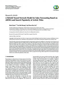
c Figure 1

Three fundamental classes of shell pigment markings on Bankivia fasciata: a, longitudinal bands; b, incremental lines; c, oblique stripes.

stimulated secretion of the mantle epithelial cells. This model differs from previous models in at least one important aspect: it depends on the "nonlocal" property of nerve nets. That is, because innervations may connect secreting cells that are not nearest neighbors, the possibility of cooperative, long-range interactions is present. This greatly enlarges the pattern-generating repertoire over nearestneighbor models, and has the virtue of relating directly to the anatomy of the mantle. Despite its simplicity, the model is remarkably successful in mimicking a wide variety of shell patterns. The paper is organized as follows. First, we catalog a number of regularities in the shell pattern that bear on the neural hypothesis. In particular, those phenomena that implicate a global organizer and preclude strictly local interactions. Second, we sketch the model equations and discuss their behavior. Third, we present patterns generated by simulations of the model and compare them to actual shell patterns. Fourth, we discuss some experiments the model suggests and some generalizations of the model. The Appendices contain the mathematical details of the model and a discussion of how it relates to other models of shell patterns.

OBSERVATIONS ON SHELL PATTERNS The variety of shell patterns is so enormous that it appears that any attempt to classify them will inevitably leave out many special cases. However, we do not hope to explain all of the patterns; rather, we seek to model the global features shared by all patterns in a restricted class. In particular, we shall focus mostly on the patterns exhibited by Nerita turrita and Bankivia Jasciata (Figures 1, 2, 3). These animals exhibit a representative variety of shell patterns from which we can draw some inferences. Many pigment patterns of gastropod shells are composites of three basic types of patterns: (a) longitudinal bands that run perpendicular to the lip of the shell, (b) incremental patterns arranged parallel to the growing shell edge, and (c) oblique patterns that run at an angle to the lines of the shell. Some mollusk taxa have more specialized types of patterns, such as the circular eye-spots on some cowry shells, or the intricate tent-like patterns on cone shells. Species differ in the categories of patterns that they display. Nerita turrita shells are always dominated by oblique patterns without longitudinal bands, whereas other members of the genus have shells with bands as well

, B. Ermentrout et at., 1986

Page 371

b a Figure 2 a, an incremental alternation in zebra stripes across the entire whorl of Bankiviafasciata; b, simultaneous termination of str! pes in B. fasciata.

as modified oblique lines. Shells of Bankivia fasciata are highly polymorphic, with various combinations of these pattern types, as illustrated in Figure 1. Longitudinal bands require only simple developmental controls. They could result from a mosaic mantle in which regions continuously deposit pigment, along with shell, separated by mantle zones that do not synthesize pigment. In general, the number and position of bands appears to be a genetic characteristic of the species, or of the individual in a polymorphic species. A second possibility-which we shall illustrate with the model-is that the band width and spacing are characteristic of the neural activity in the mantle. The two mechanisms are not mutually exclusive, as we shall discuss. Banding indicates that variation can be a permanent (e.g.) programmed) feature of the mantle edge. Incremental markings have several sources. Some appear to result from haphazard physiological stresses or environmental factors that temporarily affect the activities of the mantle as a whole. In addition, some species of snails (other than the ones we shall consider here) show regular periodic incremental shell patterns, indicating that they are programmed in a deterministic and cyclic manner. One of the most important incremental features seen on shells of the two species we have chosen for analysis are varices: time periods during which shell synthesis was halted (Figures 2, 3). In general, mollusks do not produce shell continuously, but go through cyclic periods of shell

building (producing about one-third to one-half whorl of shell in the case of Bankivia fasciata), followed by "rest" periods during which no shell is secreted. Shell patterns often are reorganized at these major interruptions in shell synthesis, and many sculptured shells produce flamboyant ridges or spines along varices. Oblique patterns are the most intricate, and have the most implications for our theoretical model. They imply that the activities involved in pigment secretion are coordinated laterally and proceed dynamically across the mantle. For example, the oblique lines shown in most of the shell illustrations in this paper represent a patch or domain of secretory activity that sweeps across the mantle, eventually migrating to its edge. These mobile domains of activity in the mantle behave in a variety of ways to produce the diverse appearance of the patterns. EVIDENCE IN FAVOR OF LONG-RANGE COORDINATION OF PATTERNS The neural network model we propose here allows for interactions and coordination beyond nearest neighbors. As we shall demonstrate in the next section, this generalization enormously enlarges the possible types of patterns over previous models, which employ short range, or "nearest neighbor" interactions. What evidence do we have that pigment secretion is indeed a neurally controlled process? We can offer no direct experimental support, for we

.....

The Veliger, Vol. 28, No.4

Page 372

b Figure 3 Abrupt reorganization of patterns on shells of Nerita turrita (a), and after a break in a shell (b).

have not been able to find any anatomical studies of mantle innervation patterns nor of secretory cell physiology. Therefore, aside from the general observation that secretory cells in most organisms are influenced by neural activity, we can offer only the following indirect evidence in support of the neural activation hypothesis of shell patterns. Global reorganizations. At a varix, a shell pattern may become systematically and simultaneously reorganized across an entire shell (cf Figures 2a, b), sometimes into an entirely different sort of pattern (Figure 3a). A variety of new patterns may arise in this manner, rather than arising locally and propagating as a wave across the shell. Such changes in the "state" of the pattern can also be initiated by a break in the shell (Figure 3b). It is hard to see how such local perturbations could have such global effects by means other than nervous activity. It should be noted that physiological and (or) environmental factors can influence the entire mantle simultaneously. Indeed, it has been demonstrated that changes in diet can alter not only the color of the pattern, but the pattern itself (D. Lindberg, personal communication). This fact does not argue for or against the neural hypothesis, for it is relatively common for dietary factors to affect nervous activity, as well as other physiological systems.

However, because diet and other environmental factors affect the pattern formed on a shell, there must be some physiological mechanism that relates the two. That is, there must be some mechanism whereby a systemic effect allows two separated regions of mantle tissue to manifest coincidental patterning. The two main avenues for transmitting stimuli from the environment to the mantle cells are soluble chemical factors (especially hormones) and nervous connections. Both may modulate patterns, but influences that differentially affect discrete parts of the mantle simultaneously seem more plausibly mediated by the nervous system. Entrainment of lines. Shells in which oblique lines become entrained in the middle of a longitudinal band also suggest coordination of pattern across sizable distances, measured in cell diameters. A particular example of this is the shell in Figure 4a, on which a band appears spaced equidistant from the neighboring bands. Termination of lines. On the shell in Figure 4b three oblique lines terminated anomalously at about the same time. These events occurred in regions of shell separated by uninterrupted oblique bands. If these changes were due to a signal that propagated from one locale to another, that signal would have to have migrated cryptically past the unaffected domains in the mantle. The simpler inter-

B. Ermentrout et aI., 1986

Page 373

I b

Figure 4 a, appearance of a band spaced equidistantly between adjacent bands; b, simultaneous termination of several separated zebra stripes without noticeable concurrent alteration of the stripes in between.

pretation is that the three separate areas were acted upon by a signal that could be conveyed to multiple local regions simultaneously. Blotching. A polymorphism (not otherwise described here) among Bankivia fasciata shells is blotching (Figure 5). On blotched shells areas of pigmentation abruptly disappear or appear incrementally across large blocks of shell. Alternatively, various segments of the mantle can be affected simultaneously by blotching. Also, for some blotched shells the zone of pigment deposition did gradually spread along the mantle, indicating that blotching can be controlled in a variety of ways. Global appearance of patterns. On some shells a general type of pattern gradually develops across the entire mantle, but with no indication that the change sweeps across the mantle; the saw-tooth pattern in Figure 6 illustrates this phenomenon. Checkerboard patterns. (Figure 7) It is possible to create a checkerboard pattern from two sets of colliding waves that propagate by strictly local interactions. However, it is remarkable that the checkerboard as a whole can stay in register without drifting in alignment. This synchronicity implies that a substantial segment of the mantle cycles back and forth between an active and inactive state in precise coordination. Adjacent subzones switch states of activity simultaneously, but in opposite directions.

THE NEURAL MODEL In this section we present a qualitative description of the shell pattern model. The mathematical discussion is given in the Appendices. The model we shall present here is the simplest possible neural model, and we do not expect (0 reproduce every shell pattern, even those observed on the two species we have selected for study. However, the model is capable of producing sufficiently diverse patterns that we consider it a reasonable first approximation; we shall suggest a number of improvements which will enlarge the class of patterns, but at the expense of computational simplicity.

BIOLOGICAL ASSUMPTIONS OF THE MODEL The basic assumption of the model is that the secretory activity of the epithelial cells that generate shell patterns is regulated by nervous activity. Specifically, we assume that the secretory cells are enervated from the central ganglion and secrete or not as they are activated and inhibited by the neural network that interconnects them with the ganglion. Although arguments in favor of this hypothesis were presented above, the issue can only be settled empirically, and experiments are under way to test the neural hypothesis directly. Figure 8 shows a schematic of the

------------........

£tQ

Page 374

The Veliger, Vol. 28, No.4

5

7 Explanation of Figures 5 to 7 Figure 5. Blotched patterns on Bankivia fasciata shells. Figure 7. Checkerboard patterns on Bankivia fasciata. Figure 6. Sawtooth patterns on Nerita tumta. mantle and the secreting cells (EMBERTON, 1963; KAPUR & GIBSON, 1967; NEFF, 1972; KNIPRATH, 1977). The specific assumptions that underlie the model are: (1.) Cells at the mantle edge secrete in intermittent (e.g.,

daily) bursts of activity. At the beginning of each session the mantle aligns with the previous pattern and extends it by a small amount. This alignment process probably depends on the ability of the mantle to sense (taste) the pigmented and (or) non-pigment-

.. B. Ermentrout et al., 1986

Page 375

extrapaZZial space periostracU7n

0000 0

shell

000

ventral epithelium Figure 8 Diagram of the anatomy of the mantle region.

ed regions from the previous period of secretion. Equivalently, a section of pigmented shell laid down during the previous period will stimulate the mantle neurons locally to continue the pattern. (2.) The secretion during a given period depends on two factors: (a) the neural stimulation, S, from surrounding regions of the mantle. (b) the buildup of an inhibitory substance, R, within the secretory cell. (3.) The net neural stimulation of the secretory cells is the difference between excitatory and inhibitory inputs from surrounding tissue. We incorporate these assumptions into the model as follows. Secretion of Pigment Depends on Current Neural Activity Consider a line of secretory cells whose position along the mantle edge is located by the coordinate x (Figure 9). Let P,(x) = the amount of pigment secreted by a cell at x during the time period t (e.g., one day). A,(x) = the average activity of the mantle neural net at position x on the mantle edge during one secretion period, t. R ,(x) = the amount of inhibitory substance produced by cells at location x in day t. S[P] = the net neural stimulation at location x during

period t. This will depend on sensing the pigment secreted during the previous period, Pt-1(x). Then the equation governing the neural activity in the mantle during period t + 1 is related to the pigment secretion during period t by the equation A/+l(X) = S[P,(x)] - R,

[ 1]

Equation [1] says that the average neural activity, +1 depends on the net neural stimulation at that location, which is stimulated by sensing the previous day's pigment S[P,(x)]. In the absence of stimulation, this nervous activity decays as the inhibitory substance R,(x) builds up. The inhibitory substance, R, builds up as pigment, P, is manufactured, and is degraded at a constant rate (0 < 1): A'+l(X), at location x on the mantle during day t

[2]

Finally, we assume that secretion of pigment will only occur if the mantle activity is above a threshold value, A *: [3]

where H(A - A *) is a threshold function for pigment secretion: It IS zero for A < A *, and one for A > A *. Equations [1] and [2] describe how the activity, A, and refractory substance, R, evolve in time; having computed A, the actual pigment secretion is given by [3]. In the computer simulations we have simplified the model even further by incorporating equation [3] into equation [1], and writing equations for P directly (ef Appendix A). This modification makes little difference in the computed

The Veliger, Vol. 28, No.4

Page 376

Figure 9 Diagram of the model: MPG, mantle pigment cells; PGN, pigment cell neurons; MNN, mantle neural net; GG, central ganglion; r, receptor cells sensing pigment laid down in time period t; P, pigment cells secreting pigment in time period t + 1; E, excitatory neurons; I, inhibitory neurons.

patterns, but is somewhat simpler to simulate. Figure 9 shows a schematic of the model's structure. Neural Activity Depends on the Difference Between Excitatory and Inhibitory Stimulation N ext, we must model the process of neural stimulation that regulates the secretion of the pigment. We regard the net stimulation of a cell at x to be the difference between excitatory and inhibitory stimulations from nearby cells. The situation is illustrated in Figure lOa: a cell located at a position x on the mantle edge received excitatory inputs and inhibitory inputs. The inhibitory signals are generally more "long range" than the excitatory inputs; that is, the mantle edge exhibits the property of shortrange excitation and long-range inhibition characteristic of neural nets (BERNE & LEVY, 1983; ERMENTROUT & COWAN, 1979). Moreover, we assume that the response of a nerve cell is a saturating function of its inputs; that is, both excitation and inhibition are sigmoidal functions of their arguments, as shown in Figure lOb. The mathematical form of the neural stimulation term we have employed is given in the Appendix. When these assumptions are incorporated into the model equations there results a set of functional difference equations that determines the pigment pattern, P,(x) (ef equations [Al, 2]). In Appendix A we perform a linear analysis on these equations. This gives some idea of the repertoire of patterns the model can generate, and provides a guide to the numerical simulations presented below.

two categories: (A) those controlling the shape of the neural stimulation function, and (B) the production and degradation rates of the inhibitory substance. Each parameter corresponds to a definite physiological quantity, and so is measurable, at least in principle. Neural parameters. The neural stimulation function, S, in equation [1] contains the curves for excitation, inhibition, and firing threshold shown in Figure 10. Each of these functions must be described by formulae that contain parameters to control their shapes. The functions we have employed in our simulations are described in Ap-

(a)

s

(b) u

The Model Parameters Any model contains adjustable parameters, and equations [1]-[3] contain several. These parameters fall into

Figure 10 Diagram of the neural influence function and threshold function.

r B. Ermentrout et al., 1986

Page 377

'." .

"'-:::""'11'5' i.:S'~Ff'1"'U":~~1:;:.ijji.W:::!iljill~WiHi~;.till;*ii:l.ri-~I~1i:i~: :;:I:Z:i'i:IWi.:!i.mitJ~~~_

~':-~,=r=~~~]j;~!Ol_~~;'itP.fc:.i:w.A.~lSlf:::jiiP.~1:'.Mii.ri.~1il!~1~lk~).;:t~;1lm.Y_~~,i:i;ru~;;.;Lt;i!.!J~jjf!~;L;jjj~~

.

~...,~_~~:t_ _:WJb.lt1L~=¥~'ti~~-=h.~~i¥:.£~~}'~e:i~~!llJi_~i~;~:'~~!~if~'!£7f~:t.';'~:-~~!i?::rg.;;;1~y'~~~.

~_ii!!!!!I~1t.:¥.~~~~~lr~!'ri~7.il~i!;*'f!!~·~F.:i1\!':~!=t"1"ri=-"~I"~i'~*;i;~~';!!,~":!;1:~;~!i\:P;~~~~:

.', ~~ .. , .... :~.~I~'l"I"I:;';;:'!~~'~"~!~'~~'of:~!;' ~!t;,.r~;r~~~·r~;r::-f':fi!~:~;~":h:;:~;l'!fi!r~~:\F:a'i~

:';'1.: '-.~:.:~:' ~-=-:-: ~·i";"~i·.• :·:.:·,·~~~!r~"'~r.:r~ln.!k~)!:'~:!l!: .. ·,,,:.\,.'::'::.r~~~~

~::~:.:.:. :.;:'~:-' :.:.:.:.:.~:. ~::~.:~:;~,::!~.:~~.:>:~~:I~:I:":: ~~:i ~':': l':'~. ~ :'~:'~':'~'::: I'~~'~':':jj~~~~~

±E~:~:~~':·;:·:~~~J~~::~;'·:··::·I:~~==~;: .,

.......

~

,' ...-···~~li~fi~Jiifif~~~;&,~ii!!iiitt~~~i;*i\i\lf~-:-··.:·::;:~.·:··...:

~iiHiiiiii~~Ii!Iii!iiiiiRii_Iiilii!iIiiiii~:a.~"'&ili*1tJl~::liiim··~~~.I'~I1-!·:~:ld~~:~:

.

1::i:i~i!UtalMm·· ~"!fi!f:t!!:l±f,t!1.1!:t!I:~~'t:t:tl·t!t·:tft.l~

Figure 11 Simulations of: a, vertical stripes of constant width; b, vertical stripes of variable width; c, horizontal stripes.

pendix A; however, experience has shown that the qualitative predictions of the model depend only on the general shapes of the functions, not on their particular algebraic form. Cellular parameters. Each secretory cell is characterized by its production rate of pigment under neural stimulation and its production and degradation of refractory substance, R. The production rate of pigment is controlled entirely by the neural stimulation, S, and so no new parameters are required to describe it. The refractory sub-

stance, however, requires the two parameters: 'Y to regulate the growth rate of R, and 0 to control the decay rate of R. Even though each of the model parameters has a direct physiological interpretation, with enough parameters one might feel that any variety of patterns is possible. However, this is not true. For a fixed neural structure, there are but two adjustable parameters: 'Y and o. Varying the neural interactions involves changes in their shape-controlling parameters, and analysis and simulation studies

a

The Veliger, Vol. 28, No.4

Page 378

1------------------~ 0:=

,

~

0

.t:I

0

-foJ

ttl

'"tj

ttl S-4 b.O

lUll

Q)

0

0 0

production of R

1

Figure 12 -y-o parameter plane showing domain of stripes and obliques.

show that the resulting patterns can be classified into a relatively small number of types. Within each distinct type, variations of the parameters merely alter the relative dimensions of the pattern, and not its qualitative appearance. However, parameter variations that exceed certain thresholds, cause the pattern to shift not just its scale, but its qualitative type as well. This "bifurcation" behavior will be discussed further below.

PATTERNS GENERATED BY THE MODEL In this section we describe the patterns generated by the neural model. We shall present numerical simulations of the neural model which mimic certain patterns observed on the shells of Bankivia fasciata and Nerita turrita. Basic Patterns Equations [1]-[3] constitute the simplest possible model for a neural net; consequently, we cannot hope to reproduce all of the known shell patterns. However, we can reproduce aU of the basic patterns; moreover, it is easy to see how the model can be elaborated to incorporate a wider variety of patterns. We shall briefly discuss these modifications here, and present a more detailed study in a subsequent paper. The three fundamental patterns exhibited by Nerita turrita and Bankiviafasciata are longitudinal bands, incremental lines, and oblique stripes (Figure 1). The parameter values that realize these patterns are given in Table 2 in Appendix A. Qualitatively, the conditions that yield these patterns are as follows. Vertical stripes (Figures la, 11) occur when refrac-

toriness is very low and the neural influence functions are strong and thresholds small. There are two mechanisms for producing stripes: one is similar to the Turing mechanism in diffusion-reaction models. That is, short-range activation creates a laterally spreading zone of activity, which is eventually quenched by the longer range inhibitory activity. This produces stripes whose width is constant, as shown in Figure lla. The stripe width is a function of the parameters (being roughly the width of the activation-inhibition zone), and the locations of the stripes are determined by the width of the domain (i.e., the size of the mantle). A different mechanism produces stripes of unequal widths, as shown in Figure llb. It is also possible to produce vertical stripes by simply activating certain regions of the mantle permanently, so that secretion is always turned on. Only experiments can distinguish between these two possibilities. Horizontal stripes, or incremental lines (Figures 1b, llc), are produced when the refractory parameters are small and thresholds are high. This results from a synchronized, or homogeneous oscillation along the entire mantle (not to be confused with the incremental pattern associated with the episodic nature of shell deposition). Diagonal stripes, or zebra bands (Figures 1c, 2, 3, 4), are characterized by very low thresholds and gradual cutoffs. These arise as waves of activity propagate along the mantle. If the neural structure is constant, the presence of oblique stripes or vertical bands depends on the values of the two parameters controlling the refractoriness, -y and o. Figure 12 shows the parameter domain that characterizes each pattern type. The direction of the stripes produced by the model depends on the parameter values. However, downward oriented stripes (i.e., away from the apex of the shell) are more common in Bankivia fasciata and Nerita turrita and exhibit far fewer irregularities. Moreover, upward-directed stripes appear to be more unstable, reverting to downward stripes after a short progression. This points to a consistent inhomogeneity in the mantle. Indeed, superimposing a parameter gradient (e.g., in 0 and [or] -y) on the model equations strongly biases the direction of striping in one direction. Interestingly, the direction of stable striping is in the same direction as the spiral of the shell. Because shell patterns are associated with shell construction, this could indicate a physiological (anatomical) correlation between the direction of shell growth and the pattern direction, such as an asymmetry in the muscle mass of the mantle. The direction of the zebra stripes can switch at certain times, especially-but not exclusivelyat a varix. Divaricate patterns. Zebra patterns may reverse directions giving a herring-bone pattern. We have used the observation that synchronous switching of the direction of stripes indicates a global coordinating mechanism for the pattern. In terms of the model, switching of the direction of obliques involves a jump in a parameter value. The model does not address what the underlying signal for

B. Ermentrout et at., 1986

Page 379

a

AAAU; +UAAAAA: AAAAAAA .AAAAAAt: :IIAAAAA AllAM.: ,IAAAAAA. IAAAAAA AAAAAAAt ·tAUAA1; •• AAAAN;, IAAAAAA+ ;AAA&. ,AAAAAU. ,AAMA%: •• • ;3AAAM, ,HAAAAAW:, ;%AAAAAAA1, :%lAAAAA%:. , ; &MAAM+. ,lAAAAAAA; : AAAAAAAt. %AAAAA%: • :3AAAAAA AAAAAAA. ,%AAAAAAAl: • : &AAAAA, ,IAAAAAAAI; :AAAAAA; AMAAAA :AAAAA'+: , ,:+&AAAAI ,+%lAMI :AAAAAAI • :IMAAAAI ;%8M AUl, +AAAAAAAI; ,%AAAAAAAAA;: .IAAMA+, ,+IAA AMI ,%AAAAAA : AAAAAAAI tMAAAAAAA, : UIAAA AAAH I; +AAAAAAAI; AAMAAA AAAAAA%, : AMAAA AAAAAI • :UAAAA ;IMMM AAAAAM+ • ;%AAAAM+ +AAAAAAU+;. tAMAIIAt:, +I; ;AAAAAIt. .AAAA!t,. ,IAAAAAAAt I&AAAAAAAL ;IAAAAAAI;. • : IAAAAA. ,IAAMAN+ IAAAAAAA+ AAAAAAI, %AAAAAI:. :SAAAAAA: :$AAAAAA AAAAAAAA tlAAAAAAAI .IAAAAAAiI+, AAAAAA: ,AAAAA&+ MMAAU;, , .: %AAAAA, •• alAAA+,. :%AAAAAI ,UAAAAAAA+ :%&U +. AAll, IAAAAAA%, ; lAAAAAAA.; ; AMAAS: ,lAM AAAI, ; MAAAAAA. ;AAAAAAAI +AAAAAAAI ,tlAAAA MAn: IAAAAAAA1, AAAAAAA AAAAM.: ,AlIMA' AAAAA&. ,;$AAAAM SAAAAAI :AAAAAAA; .;XAAAAU+ ;IAAAAAU+, &AAAAA$:.. ;&U: SAAAA1+: ,AMA';, .. • ;SAAAAl :$AAAAAAMt. +lAAAAAAAS .+IAAAAAAI; : IAAAAAI+ &AAAAAAAt ,AAAAAAA; :AAAAAI:. :HAAAAA: ,IAAAAAA AAAAAAAA ,%AAAAAAAf .&AAAAAAUt, .AAAAAA, .AAAAAA$ ;AAAAAlt; , ., ;IAAAAA. ,XSUMt. ,1AAAAAA: ;UAAAAAA& + .;131 AU+, ,MAAAAAA%, ; MAAAAAAAM;, • AAAAA&;. .+lAA AAAI. ,l!lAAA ;WAAAAAA ;AAAAAAA& tMAAAAAAA, AAA&% , IAAAAAAAL AAAAAAA AAAAAAS: ,AAAAAA AAAAH. ,+&AAAA& lAAAAA& :AAAAAAA+ :+IAAAAA1 +IAAAAAUt, MAAAH, •• !AAAAAl:. +UI: %AAAAl+:. .; IAAAAS ,SA AAAAA&+. HAAAAAAAI • +&AMAAA1+, :IAAAAAM+ MAAAAAAA+ .AAAAAAA; SAAAAA%: • : &AAAAAA AAAAAAAA • UAAAAAAI • :%AAAMA, ,AAAAAA$+ • ,!AAAAAAUi· ,AAAAAA, • AAAAAAI , : IUAAA: +AAAAAA; ,UAAAAAAM • ;%$1 • ,'SMAAa AU+. : AAAAAAA+, .IAAAA&;. ;IAA • ;&AAAAAAAMt: ,ZUMA AAM. .;MAAAAAM +AAAAAAA& ; MAAAAAAA, AAAU: SAAAAAAA% • AAAAAAA AAAAAA&; ,MAAAAA AAAAAI. :+AAAAA+ SAAAAA& • MAAAAAA! • ;&AAAAAI tAAAAAAU; • ·.AAAAAA+, • %AAI+ jAAAAM%;, lAAAU i, . , ; lAAAA+ ; SAAAAAAS;. ;nAAAAAAI. .+&AAAAAAMt : ; IAAAAA&; • MAAAAAAA+ %AAAAAl: • • AAAAAAA+ • • ,%AAAAAA. +IAAAAAAI ; MAAAAAA &AAAAAAA : HAAAAAU: +AAAAAA. AAAAAAl. , AAAAAAU, ,: IlAAAAI ;SIIAAl, :AAAAAA% : +lAAAAAAA; :+SI AU; +AAAAAAIt • : tlAAAAAAAA+; • lAMA!; • :%MA AAM+ • HAAAAAl ;AAAAAAA& : &AAAAAAA: :I&lAAA AAAf%: &AAAAAAA+ IMAAAN+ • ,IAAAAA AAAAAAA, AAAAAt. .: IAAAAA, &AAAAAM , &AAAAAAA : IAAAAAI IAAAAAU+ : ;AAAAAA; • &AAA$ ;AAAAZ;: , :AAAAIl; , .+1AAAAA.+;. ,+MAAAA, • +&AAAAAAU: : tSAAAAAAM, : MAAAAAAA+ &AAAAAAZ, IAAAAAZ: • • +AAAAAAI; ; MAAAAAA ZAAAAAAA: ; !AAAAAAL %AAAAAA ;!AAAAAAH, MAAAAAA AAAAAAX, AAAAAA*l:

b ':

Figure 13 a, divaricate patterns on Bankivia fasciata showing open and closed V's; b, simulation of V's.

such an event is, but does provide a mechanism for generating a coordinated reversal of the pattern orientation (Figure 13). Lines that converge as the shell grows will be called "closed V's"; those that diverge as the shell grows are "open V's." Pattern reversals that produce a "closed V" frequently extend beyond the intersection a small amount, forming a "snout" on the V. This is also a feature of the simulations, because a collision of two obliques admits a small overlap of the activation region extending' beyond the collision apex. Note also that the upward stripes are shorter than the downward stripes, suggesting a mantle inhomogeneity. This has been suggested previously by WRIGLEY (1948).

Wavy stripes (Figure 14). These are characterized by very sharp cutoffs of the excitatory and inhibitory thresholds, small thresholds, and large turnover of refractory substance ('Y, a"" 1). Note the "shocklike" discontinuities in the stripes that the simulation reproduces. Streams (Figure 15) are irregular striped patterns that occur when the sharpness of the cutoff is quite large and refractoriness is persistent (0 "" 0.8). Interaction Patterns In addition to the basic patterns, additional designs emerge from the interaction of the basic patterns. Typi-

Q

The Veliger, Vol. 28, No.4

Page 380

,+UA'+i;aU& %AAAAAUU, XAAA+ii •• ·ij:j;:;;i: UAAI , •• AU;, +UA :AAl" ;'AAAtj~ +IX, •• , .SUAA :i; i:IAIl ,+.AAAAi ::A%%:&lA;, ,:AAAAJ, ,,+IAAAA%: lAAAAA. :AAAA., :;Ulij;jij;ij ,. UAUAt: iUS: .AAAAA, jj% :+AAAI,.,+UAAAUAUAUll AAAA%: :IAUA';: +U;: :jAAAl+ .jAAAj;+IU%%IIAIAAAAAI:; AU: :AAAAAAAAA AAAAAAA&; :AAAAA%% +%%%U%lAAIIAI;: .. :UAAA;:&AAA+ +UAAAAAAI :IAUS, "UI".IAAAAA :fAAAA' :AAA,. ::AAa •• jAAAAI; UI1.::: ••• i. :.AAA :SAAAAA. "AAAUAA, • jAAAAI: ,j :Ul:: :lIA • ,.AAAAA+. "AAAAAAA jAAAAA: %AAAU, ,++XI. .+ +AIIAAA+. ,&AA%; .AAAAI. ++1 .+AAAAS AAAAAAlj.AAAA&; AAAA+. +AAAAAAj .:. ifAAU+ ;AAAA; I:;:UUIIAAAAA;. AA&. .+AAAAAAAAI AAAAAAU: .AUAAI ;. US+,. jAAAAl, t, .+AAAA, %AAA+ +AAAUUAAI. .+AUA lAI. jllAAAA • +AAMA. • &AAX j: +IAA+ lUAA:, ,SAA, j :; ,: I,. :$AAA (JE, and since the local excitation strength is generally greater than the inhibition, we choose OlE > Oil' The responses of the secretory cells to neural stimulation are assumed to be sigmoidal functions of their inputs: S[P'(x)J = SE[E,+Jx)J - SAI'+l(X)J

[10]

For simulation purposes, we have employed the following function for both S E and S / S(u)J

1

+1

e",Iu-Oj) ,

)=E,/

[11]

B ~~---l-_=:;::) A ---I'---+--+---b

(c)

c Figure Al

a, the unit circle and the stability triangle on the coefficient (a, b) plane; b, dispersion relation A(k) for spatial instability; c, trajectories for each type of bifurcation.

where we have suppressed the dependence on x for notational simplicity. Let Po be a homogeneous equilibrium, i.e., Po = S[PJ

The parameter v) controls the sharpness of the nonlinearity, and OJ the location of the threshold. Thus the raw parameter list consists of the 12 quantities:

This list can be reduced to nine because some parameters enter only as products, and some may be rescaled. Table 1 summarizes the model parameters.

+ oPo - (-yP o + oS[PoJ)

[13J

or

1- 0 Po = S[PJ 1 - 0 + 'Y

[ 14J

If we shift the sigmoid S so that SIlO) = SlO) = 0, then we can linearize about Po = 0 to obtain the linear difference equation:

Pt+2

+ L,p,+! + oP,

- [yP,

+ aLo(p,)J

=

0

[15]

where L,(.) is the linear (convolution) operator

B. Analysis and Simulation of the Model A linear stability analysis of the model equations gives some idea of the patterns the model will generate. Therefore, we proceed as follows. The pair of equations [4, 5] are equivalent to the single second order equation

[12]

L,luJ(x) = S'E(PJ

1

- S'/(P,,)

WE(x' - x)u(x') dx'

I

W/(x ' - x)u(x ') dx ',

where S'iP,) are derivatives of SJ.

[16J

Q

I

The Veliger, Vol. 28, No.4

Page 386

,..--+--+---'r--, X

1

(a)

(b)

Ot----------k Figure A2 a, the shapes of S(x) and L(k); b, the dispersion relation.

On a periodic domain of length L (e.g., the limpet), the eigenfunctions for La are exp(27f"inx/L), n = 1,2, ... ; on a finite linear domain these are approximate eigenfunctions, since the domain size, L, is much greater than the range of the connectivity functions W. The characteristic equation for the spatially homogeneous system is obtained by substituting P,(x) :::::: >"'exp(27f"ikx/L) into the linearized equation: >.,2 + (L *(k) + 0»).. - ['Y + 5L *(k)]

==

)..2

+ a(k»)" +

b(k) = 0

[17]

Here L*(k) == S'E(Po)We(k) - S'/(Po)W/(k)

[18]

where the ~ are (close to) the Fourier cosine transforms of the ~:

~(k) ::::::

1

cos(27f"kx/ L)

~(x) dx

[19]

The spatially homogeneous solution is stable if and only if the roots of the characteristic equation lie within the unit circle on the complex plane: I).. I < 1 for every k = 0, 1, 2, .... This condition can be plotted on the coefficient plane (a, b), as shown in Figure Ala, where stability requires that a and b lie within the shaded triangle. Spatial instability requires that (i) the homogeneous solution be stable: I).. I (k = 0) < 1, and (ii) there exists a

t

/Al

__ __________

~'A~

finite range of unstable modes: I).. I (k) > 1 for a < k1 < k < kz < 00. That is, the dispersion relation )"(k) should look qualitatively as shown in Figure Alb. Such an instability can arise in three qualitatively different ways: as one of the model parameters is varied the unstable eigenvalue can pass out of the unit circle through +1, -1 or at a complex value (Figure Alc). Which one of these instabilities occurs depends on which parameter is varied and on the shape of the connectivity kernels, W)" The neural connectivity function, W(x) we have employed is the usual "short-range excitation/long-range inhibition" type shown in Figures 9 and 10. The linear operator L*(k) is essentially the Fourier transform of W(x). By the properties of the Fourier transform, L *(k) has the shape shown in Figure A2a. Because only positive values of k are physically relevant, the dispersion relation looks qualitatively as sketched in Figure A2b. The three paths to spatial instability shown in Figure Alc correspond to violating the following three inequalities: (a) Bifurcation through +1 will occur if L*(k) > (1 - 'Y)/5 (path a in Figure Alc). This is a so-called "equilibrium" bifurcation because in the spatially homogeneous case (k = 0) such a bifurcation creates a new equilibrium point (cf MAY & OSTER, 1976; GUCKENHEIMER et at., 1976). When k > a this creates a stationary spatial pattern of regularly spaced stripes as shown in Figure A3a. (b) Bifurcation through -1 will occur if L *(k) < -(1 + 'Y/(1 + 5» (path b in Figure A1c). From Figure A2b we see that this can occur only at k = 0, so that homogeneous instability results. (This can only happen in this model for the kernel shown providing 8Jo; ~ 8I> since we have assumed that at: > a/.) The pattern resulting from this bifurcation consists of fine horizontal stripes, as shown in Figure A2b. (c) Bifurcation through A = e iO (8 .,. 0, 7f") occurs if L*(k) > 1 + 'Y/(1 - /J) (path c in Figure Alc). This generates periodic spatia-temporal patterns, as shown in Figure A3c (e.g., stripes and checks). Note that (1 - 'Y)//J < 1 + 'Y /(1 - {j) if and only if {j > 1 - Vi Thus + 1 bifurcations occur first when /J < 1 - 'v0; otherwise the bifurcation is via a complex eigenvalue. When 'Y = 0, so that the refractory substance cannot build up, the model can take a particularly simple form. If we make p large, and (J E, (J / equal, and v large, then the model is approximated by the rule: P'+I(X)

=

1 if 8E
D A). He obtained some of the same patterns we obtain here by assuming that each cell of the automata could periodically fire and become refractory for a while. In a more recent simulation, Meinhardt and Klingler (to appear) included longer range interactions by allowing morphogens to diffuse beyond nearest neighbors. These simulations resemble ours and it appears that most patterns can be created by either mechanism. However, it is not clear how the diffusion-reaction model handles the problem of pattern alignment between episodes of shell secretion, whereas this is intrinsic to the neural model. Wolfram's simulations mimic to a remarkable extent the "tent" patterns observed on many cone shells. However, his rules were rather arbitrary, and have no obvious physiological interpretation. The neural net model, in the limit of short-range interactions and sharp threshold functions, reduces to the automata model, and can also reproduce the tent patterns. All of these models have a similar structure: a locally excitable activator-inhibitor system that is coupled spatially to nearby points. In order to obtain spatial patterns, the activation-inhibition is essential. Moreover, it appears that many of the patterns depend on the long-range (i.e., beyond nearest neighbor) interactions characteristic of neural nets. Also, the episodic nature of the secretion process dictated our choice of a discretized model in time; this feature also appears essential to the formation of certain pattern types. In a subsequent publication we shall investigate a broader class of neural models, including kernels with long-range activation and two-dimensional mantles, such as are found in cowries.