A Model of BGP Routing for Network Engineering Nick Feamster Jared Winick Jennifer Rexford MIT Computer Science & AI Lab Lockheed Martin AT&T Labs–Research
[email protected] [email protected] [email protected]
ABSTRACT The performance of IP networks depends on a wide variety of dynamic conditions. Traffic shifts, equipment failures, planned maintenance, and topology changes in other parts of the Internet can all degrade performance. To maintain good performance, network operators must continually reconfigure the routing protocols. Operators configure BGP to control how traffic flows to neighboring Autonomous Systems (ASes), as well as how traffic traverses their networks. However, because BGP route selection is distributed, indirectly controlled by configurable policies, and influenced by complex interactions with intradomain routing protocols, operators cannot predict how a particular BGP configuration would behave in practice. To avoid inadvertently degrading network performance, operators need to evaluate the effects of configuration changes before deploying them on a live network. We propose an algorithm that computes the outcome of the BGP route selection process for each router in a single AS, given only a static snapshot of the network state, without simulating the complex details of BGP message passing. We describe a BGP emulator based on this algorithm; the emulator exploits the unique characteristics of routing data to reduce computational overhead. Using data from a large ISP, we show that the emulator correctly computes BGP routing decisions and has a running time that is acceptable for many tasks, such as traffic engineering and capacity planning.
Categories and Subject Descriptors C.2.2 [Network Protocols]: Routing Protocols; C.2.6 [ComputerCommunication Networks]: Internetworking
General Terms Algorithms, Management, Performance, Measurement
Keywords BGP, traffic engineering, modeling, routing
1.
INTRODUCTION
The delivery of IP packets through the Internet depends on a large collection of routers that compute end-to-end paths in a dis-
Permission to make digital or hard copies of all or part of this work for personal or classroom use is granted without fee provided that copies are not made or distributed for profit or commercial advantage and that copies bear this notice and the full citation on the first page. To copy otherwise, to republish, to post on servers or to redistribute to lists, requires prior specific permission and/or a fee. SIGMETRICS/Performance’04, June 12–16, 2004, New York, NY, USA. Copyright 2004 ACM 1-58113-664-1/04/0006 ...$5.00.
tributed fashion, using standardized routing protocols. Providing low latency, high throughput, and high reliability requires network operators to adjust routing protocol configuration when performance problems arise or network conditions change. For example, an operator might adjust the configuration to respond to network congestion or equipment failures or to prepare for planned maintenance. However, the complexity of the protocols, the large number of tunable parameters, and the size of the network make it extremely difficult for operators to reason about the effects of their actions. The common approach of “tweak and pray” is no longer acceptable in an environment where users have high expectations for performance and reliability [1]. To avoid costly debugging time and catastrophic mistakes, operators must be able to make predictions quickly based on an accurate model of the routing protocols. Previous work in this area has focused on Interior Gateway Protocols (IGPs), such as Open Shortest Path First (OSPF) and Intermediate System-Intermediate System (IS-IS), that operate within a single Autonomous System (AS). In these protocols, each link has a configurable integer “cost” that is used to compute the shortest path (smallest cost path) through the network. Tuning these link weights gives operators a way to modify the paths inside the AS to satisfy network and user performance goals [2]. Several existing tools [3, 4, 5] capture how changes to the link weights would affect the flow of the offered traffic over the new paths and also propose good candidate settings of the link weights. Although these tools are extremely valuable to network operators, the flow of traffic in large service provider backbones ultimately depends on the interdomain routing protocol as well. A provider uses the Border Gateway Protocol (BGP) to exchange reachability information with neighboring domains and to propagate these routes within its own network. Unfortunately, several subtleties make modeling BGP route selection in an AS much more challenging than emulating IGP: • BGP’s distributed, path vector operation means that every router may have a different view of network state. In contrast to link state protocols that flood complete information throughout the network, a BGP-speaking router sends incremental reachability information only to its immediate neighbors. In BGP, a router sends an advertisement to notify its neighbor of a new route to a destination prefix and a withdrawal to revoke the route when it is no longer available. Each BGP-speaking router locally computes its own best BGP route from the best routes announced by its neighbors. A change in the best path at one router can affect the selection of the best route at another router, and no single router has a complete view of the available BGP routes in the AS. • BGP route selection is a complex process that depends on a combination of route attributes. While most IGPs advertise a single integer metric for each link and select routes based on shortest
Neighboring AS eBGP routes
a
A
b
egress routers
eBGP routes
B
R
ingress router
Figure 1: Network engineering terminology.
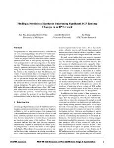
paths, BGP route advertisements include various attributes, such as the list of the ASes in the path (the AS path) and the IP address of the router responsible for the route (the next hop). BGP route selection is based on a complex, multi-stage decision process [6]. BGP allows operators to specify complex policies that have an indirect effect on the selection of the best path. • BGP route selection depends on interactions with intradomain routing protocols. Whereas the IGP can be modeled in isolation, the selection of the best BGP route at each router also depends on the IGP path cost to the BGP next hop announcing the route. “Hot potato” routing, where a router prefers the route with the shortest IGP path (the closest exit point), introduces a complex coupling between BGP and the underlying IGP. • Hierarchical iBGP configuration affects the routing choices that are available at each router. Internal BGP (iBGP) is used to distribute BGP-learned routes throughout an AS. Rather than having an iBGP session between each pair of routers (“full mesh iBGP”), large provider networks typically distribute routes in a hierarchical fashion. This makes the choices available at one router dependent on the decisions made at other routers and may prevent the protocol from converging. In this paper, we present a model that accurately determines how the network configuration and the routes learned via external BGP (eBGP) affect the flow of traffic through an AS. While some existing tools simulate BGP’s behavior [7], this is the first paper to develop a model that determines the outcome of the BGP path selection process at each router in an AS without simulating the dynamics of the protocol. This type of model is important for several reasons. First, network operators need to know the paths that routers ultimately select to perform engineering tasks (e.g., traffic engineering and maintenance), but they have no need for a computationally expensive simulation of routing dynamics. We present an emulator based on our model that facilitates these tasks by providing fast, accurate answers to “what if” questions about the effects of changes to the network. Second, an accurate model of BGP route selection can be used to improve and validate existing simulators by highlighting subtleties of the protocol and situations where BGP might not converge to a unique solution. A simulator may only compute one possible outcome, which may not accurately reflect the outcome in a real network. The modeling framework we present can determine whether a BGP configuration would converge to a unique outcome. Predicting how a configuration change would affect the flow of traffic first requires a way to determine which route each ingress router in the AS would select for each destination prefix, given a network configuration and the eBGP routes learned at the egress routers (as shown in Figure 1). This paper solves precisely this problem. The model of BGP routing that we present is essentially an abstraction that conceals protocol details that are irrelevant to the outcome of the BGP decision process. The model computes
BGP routing decisions when the network is configured “correctly”, which can be checked separately by testing certain sufficient conditions. Our model can also be combined with prefix-level traffic measurements to form the basis of a traffic engineering tool. The rest of the paper is organized as follows. In Section 2, we present several examples of network engineering tasks that motivate the need for an accurate, predictive model of BGP path selection in an AS. Section 3 describes the practical constraints that the network configuration and routing advertisements must satisfy to make modeling BGP route selection possible and applies these constraints in a novel way to decompose the route prediction problem into three distinct phases. In Section 4, we describe each phase of the route prediction algorithm in detail. Section 5 describes a prototype implementation of a BGP emulator. In Sections 6 and 7, we present an evaluation and validation of our prototype on routing and configuration data from a large tier-1 ISP. These experiments show that the route prediction algorithm accurately predicts BGP routing decisions and that it is efficient enough to be practical for many network engineering tasks. Section 8 provides an overview of related work. We conclude in Section 9.
2. NETWORK ENGINEERING In this section, we discuss network engineering problems that operators commonly face. These examples demonstrate the need to systematically model BGP’s route selection process and move beyond today’s “tweak and pray” techniques. We then discuss why a practical model of BGP is useful; in particular, we discuss the advantages a model has over simulation and live testing.
2.1 Network Engineering Problems Network operators must adjust routing protocol configuration to respond to the following common changes in network conditions: • Changes in traffic load. Because traffic is dynamic, the amount of traffic to any destination may suddenly change, causing changes in traffic distribution across network links. For example, a Web site sometimes experiences a traffic surge due to a flash crowd (i.e., the “Slashdot effect”); a network that was routing traffic to that destination through a neighboring AS could experience congestion on an outbound link to that destination. A network operator must reconfigure routing policy to alleviate congestion. • Changes in link capacity. Network links are frequently upgraded to higher capacity. In response, network operators may wish to adjust configuration to route additional traffic through recently upgraded links. For example, if link a in Figure 1 were upgraded from an OC12 to an OC48, a network operator would want to shift traffic from b to a. • Long-term connectivity changes. On longer timescales, the points where a network connects to neighboring ASes, as well as the ASes that it connects to, change. As links to other ASes appear and disappear, network operators must move large amounts of traffic. If the AS shown in Figure 1 added a third link to its neighboring AS, an operator would shift a portion of traffic to that AS from a and b to the new link. • Changes in available routes. Due to protocol dynamics and changing commercial agreements, an AS might suddenly receive an alternate route to a destination that could cause traffic flow to shift dramatically; alternatively, an existing route could suddenly disappear. These events may require a network operator to rebalance the flow of traffic. • Planned maintenance. Network operators commonly perform routine maintenance on portions of their network, adjusting inte-
rior routing link weights to divert traffic away from the part of the network that is undergoing maintenance. If router R were undergoing an upgrade, the network operator could adjust both the IGP link weights and the BGP configuration to divert traffic away from R without overloading links that border neighboring domains. • Failure and disaster planning. An operator may wish to evaluate the robustness of the network by examining the effects of failures on routing and traffic flow. Studying the effects of a component or link failure or even a more serious catastrophe (e.g., fiber cut, tunnel fire, or terrorist attack) helps network operators and planners make design decisions. Tools exist to help network operators adjust interior routing protocol parameters to rebalance traffic within an AS [3, 4, 5], but operators must also rebalance traffic across its external links to other networks by reconfiguring BGP. A network operator who wants to shift traffic from link a to b in Figure 1 typically would adjust the import policy for a set of routes at router A, commonly by decreasing the “local preference” attribute that router A assigns to these routes [8]. This would cause the routes learned at router B for these destinations to appear more attractive than those at A, causing the traffic to those destinations to exit the AS via B.
2.2 Network Engineering Requirements Motivated by these practical network engineering examples, we now present several requirements for a network engineering tool that predicts the outcome of BGP route selection. (Throughout the paper, we use the term “prediction” to describe the process of determining the outcome of BGP route selection offline.) • Operators need to be able to predict the effects of a configuration change before deployment in the live network. Operators typically handle network engineering tasks by tuning the existing configuration of the live network, witnessing the effects of the change, and reverting to the previous configuration if the desired effects are not achieved. This method is time consuming and can lead to unnecessary performance degradation. The complexity of interdomain routing makes it essentially impossible to compute back-ofthe-envelope estimates of the effects of configuration changes. • Because network engineering involves exploring a large search space, operators need to predict the effects of each candidate configuration change as quickly as possible. Operators usually need to experiment with many possible configuration changes before arriving at an acceptable solution. This requires techniques for quickly evaluating the effects of a proposed configuration change. In practice, the candidate configuration changes typically are just small modifications to the existing configuration, which are less likely to cause significant unexpected changes in routes or the offered traffic load. To be useful, a route prediction tool should be fast at evaluating incremental changes. • Network engineering tasks require an accurate prediction of the outcome of the BGP path selection process but do not require a detailed simulation of the protocol dynamics. Network simulators (e.g., SSFNet [7]) help operators understand dynamic routing protocol behavior, but simulation represents network behavior in terms of message passing and protocol dynamics over a certain period of time. In contrast, network engineers usually just need to know the outcome of the path-selection process and not the low-level timing details. Furthermore, existing simulators do not capture some of the relevant protocol interactions that can affect the outcome of the decision process. Simulating every detailed interaction is hard to do without a higher level model of BGP in the first place. In summary, BGP path selection is a massive, highly tunable, distributed computation. To maintain good end-to-end performance,
operators need a way to predict the outcome of this computation under various configurations (1) efficiently, (2) in a way that facilitates evaluating incremental changes, and (3) without deploying configuration changes on a live network. In the following sections, we describe a way to model the BGP decision process across every router in an AS; our algorithm correctly and efficiently computes the outcome of the BGP decision process at each router.
3. MODELING FRAMEWORK At a glance, modeling the routing decisions in an AS seems as simple as applying the BGP decision process at each router. However, the BGP routing system inside an AS is not guaranteed to converge to a unique solution where routers make consistent decisions. Even when the system converges, the decision made at one router can affect the options available to other routers. Applying theoretical results from previous work, we impose three practical constraints on the routing system that make modeling BGP route selection possible. We then show that route selection can be modeled in three distinct phases when these constraints are satisfied.
3.1 Constraints on the Routing System Given the eBGP-learned routes to a destination prefix, we would like to determine which route each router would ultimately select. Unfortunately, certain network configurations do not lend themselves to efficient route prediction. This is a fundamental problem underlying BGP—some configurations do not converge, and determining whether a system converges to a unique solution is computationally intractable [9]. To make modeling BGP route selection feasible, we impose three constraints and explain why these constraints are reasonable to assume in practice. If the eBGP-learned routes change frequently, the internal routing system does not have time to propagate the effects of one eBGP advertisement before the next one arrives. As such, we assume: C ONSTRAINT 1. The eBGP-learned routes change slowly with respect to the timescale of network engineering decisions. In practice, most BGP routes are stable for days or weeks at a time [10], and the vast majority of traffic is associated with these stable routes [11]. This allows emulation to operate on a static snapshot of the eBGP routes. Any eBGP routing change can be treated as a separate problem instance. Network operators have significant flexibility in deciding how to propagate the eBGP-learned routes throughout the AS. In the simplest case, the routers are configured in a full mesh of iBGP sessions. In general, though, the routers may form a more complicated signaling graph of iBGP sessions, as shown in Figure 2. Each edge corresponds to an iBGP session between a pair of routers. A router does not normally forward iBGP-learned routes to its other iBGP neighbors. However, a router can be configured as a route reflector (RR), which forwards routes learned from one of its route-reflector clients to its other clients. Following terminology from previous work [12], we use the term up for the iBGP session from a router to its RR, over for a conventional iBGP session between two routers, and down for the iBGP session from an RR to a client. A valid signaling path consists of zero or more up edges, followed by at most one over edge, followed by zero or more down edges. Alternatively, routers within an AS can also be grouped into one or more “confederations”. Because confederations are used much less frequently than route reflectors, we focus on modeling route reflectors and do not model the effects of confederations. Every eBGP-learned route should propagate through the signaling graph to every other router in the AS. For example, consider
1. 2. 3. 4. 5. 6. 7.
over
RR2
RR1 over down
W
X
Y
up
Z
Highest local preference Lowest AS path length Lowest origin type Lowest MED (with same next-hop AS) eBGP-learned over iBGP-learned Lowest IGP path cost to exit point Lowest router ID of BGP speaker2
Figure 2: Example iBGP signaling graph
Table 1: Steps in the BGP decision process
Figure 2. The edge between RR1 and RR2 is an over session, whereas the edge from Z to RR2 is an up session. An eBGP route learned at Z can reach Y via RR2 and RR1. An AS’s signaling graph can violate this property even if all routers are connected via IGP. For example, if the session between Y and RR1 were an over session instead of an up session, Y would have no way to receive an eBGP route learned at Z. These types of partitions can make modeling difficult; therefore, we assume:
which prevents “deflections”. Part (c) is more difficult to ensure in practice but is consistent with the approach of assigning clients to RRs that are along the shortest path to each egress point. Imposing these three constraints make modeling BGP route selection possible. Each router applies a multi-stage decision process [6] to select a single best route, as summarized in Table 1. The decision process considers the set of available routes to a destination and proceeds step-by-step to eliminate candidate routes. For example, the decision process first eliminates all routes that do not have the highest local preference value, and so forth, until a single best route remains. Since the route selected at one router can affect the routes available at another router, we cannot simply apply the BGP decision process independently at each router. Although we must model the distribution of routes within an AS, Constraints 1 and 3 ensure that the system converges to a unique solution, which allows us to apply the following intuitive result:
C ONSTRAINT 2. Each router has a valid iBGP signaling path to every other router1 . An operational network should not violate this constraint, since this could create a network partition, even though the AS is connected at the IP level. An AS with a full mesh of iBGP sessions satisfies this constraint; so does a full iBGP mesh among the top-level RRs who, in turn, each have iBGP sessions to their RR clients (a common configuration scenario). Ensuring that each eBGP-learned route has an iBGP path to every other router still does not guarantee that each router converges to a unique solution. A router only learns about the routes advertised by its immediate iBGP and eBGP neighbors. For example, in Figure 2, if W and Z have eBGP-learned routes, router Y learns a single route from its route reflector RR1. Suppose that RR1 selects the eBGP route advertised by Z. Then, Y would pick Z’s route as well, even if Y would have preferred W ’s route over Z’s route. Note that Y makes a different routing decision than it would if it could select its best route from all the eBGP routes (i.e., from both W and Z). In some situations, differences in the routers’ local rankings of the BGP routes can cause persistent oscillations and even forwarding loops, which make it difficult to model the outcome of the BGP decision process. Fortunately, these problems can be avoided if the network configuration satisfies the following sufficient condition [12]:
T HEOREM 1. If a routing system is guaranteed to converge to a unique solution, the solution is independent of the order that routers exchange routes and apply the decision process. We proved a slightly different version of this theorem in our previous work (Theorem 4.1, [13]). In practice, a router may receive numerous route advertisements and select (and propagate) a best route multiple times before settling on a final choice. Fortunately, with careful selection of a particular ordering of these events, a prediction algorithm can predict the outcome without simulating the protocol dynamics.
3.2 Phases of the Route Prediction Algorithm
Part (a) is satisfied when routers do not change the attributes of iBGP-learned routes and each router has a lower IGP path cost to its clients than to other routers. The common practices of applying import policies only on eBGP sessions and placing RRs and their clients in the same point-of-presence (i.e., “PoP”) ensure that these conditions hold. Part (b) states that if a is an RR for b, and b is an RR for c, then c is not an RR for a, consistent with the common practice of constructing a route-reflector hierarchy, rather than an arbitrary signaling graph. Part (c) ensures that all routers along a shortest path to an egress point have selected the same egress point,
Although some of the constraints we discussed have previously been presented as conditions for stable routing, these constraints are also necessary to model BGP route selection; we now constructively apply these constraints to propose a novel way of decomposing route prediction. Theorem 1 gives us the flexibility to define a message ordering without affecting correctness. Specifically, the algorithm selects a message ordering that decomposes the problem into three distinct phases, as shown in Figure 3. The rest of the section explains this decomposition, deferring the detailed discussion of each phase to Section 4. Receiving the eBGP routes and applying import policy: The first phase assumes that each router receives all of its eBGP-learned routes and applies the import policies, before exchanging any iBGP update messages. Each eBGP-learned route has attributes (such as the destination prefix and the AS path) and is associated with an eBGP session. The import policy may filter the route or set certain attributes such as local preference, origin type, and multiple-exit discriminator (MED), according to attributes in the advertised route (e.g., based on ASes in the AS path). Because applying the import policy is a local operation for each eBGP-learned route at each
1 This
2 Some
C ONSTRAINT 3. (a) A router prefers routes learned from down neighbors over routes learned from other neighbors, (b) the signaling graph does not have any cycle of up edges, and (c) the shortest IGP path between each pair of routers is a valid signaling path.
property can be checked by a breadth-first walk through the edges in the signaling graph and marking the nodes as they are visited; in the graph walk, an over or down edge can only be followed by a down edge.
router vendors allow tiebreaking based on the “oldest” route (i.e., the route that was learned first). This feature is often disabled to avoid introducing non-determinism into the BGP path-selection process.
eBGP routes (per prefix)
import policies
router ID
(per eBGP session)
(per session)
Apply import policy
modified eBGP routes (per prefix)
Compute best eBGP routes
iBGP signaling graph
IGP path costs (per ingress−egress pair)
best eBGP routes (per prefix)
Compute best BGP route
best egress point (per prefix & ingress)
Figure 3: Decomposing network-wide BGP route selection into three independent phases router, the first phase emulates exactly the operations a real router would perform upon receiving each of the eBGP routes. These routes, with modified attributes, form the input to the second phase. Computing the best eBGP-learned routes: Many routes from the first phase would never be selected by any router as the best BGP route. For example, an eBGP-learned route with a local preference of 90 would never be selected over another route with a local preference of 100. As long as every eBGP-learned route can reach every router (Constraint 2), no router would ever make a less attractive decision than any other router in the AS. In other words, C OROLLARY 1. Constraint 2 implies that every router in the AS selects a best BGP route that is equally good through the first four steps in the decision process. For example, a router on the east coast of the United States might select a route learned in New York, whereas a router on the west coast might select a route learned in San Francisco. Still, these two routes would have the same local preference, AS path length, and origin type; if the two routes have the same next-hop AS, they would also have the same MED value. This property allows the second phase of the algorithm to focus on the selection of the “best” eBGP routes across the eBGP-speaking routers, without modeling the details of distributing these routes throughout the AS. Modeling the influence of iBGP and IGP within the AS: In the third phase, each router selects a single route from the set of best eBGP routes. Each border router that contributes to the set of best routes selects its own best eBGP-learned route. Every other router selects one of these routes after they have propagated via iBGP; this behavior is consistent with step 5 of the BGP decision process. The decision at each router depends on the routes selected by its iBGP neighbors, the costs of the IGP paths to the exit points where these routes were learned, and the router IDs of the iBGP sessions. This introduces a dependency between iBGP and IGP. Fortunately, the algorithm only needs to consider the total IGP path cost of the shortest IGP path(s) between each pair of routers, rather than hop-by-hop costs. We can make this simplification because Constraint 3(c) implies that all of the routers along the IGP path from a router to its chosen egress point have selected the same best BGP route. That is, no router along the path to the egress point would deflect a data packet toward a different egress point than the ingress router had selected. Although the diagram in Figure 3 shows only three phases, we envision that network operators could incorporate other modules for additional functionality. For example, a module could combine the predicted BGP routes with traffic data to predict the load on each link in the network. Using the emulator for traffic engineering assumes that traffic volumes are relatively stable, and that they remain stable in response to configuration changes. In previous work, we found that prefixes responsible for large amounts of traffic have relatively stable traffic volumes over long timescales [8]. Operators could use the emulator to test configuration changes on reasonably slow timescales that affect prefixes with stable traffic
volumes. A network operator could also combine measurements or estimates of the traffic arriving at each ingress point for each destination prefix [14] with the link-level paths to predict the load on each link in the network. Another module might evaluate the optimality of the these link-level paths in terms of propagation delay or link utilization and could search for good configuration changes before applying them on a live network.
4. ROUTE PREDICTION ALGORITHM Drawing on the modeling framework from Section 3, this section proposes an algorithm that computes the best route at each router in an AS. Since the path selection process is independent for each prefix, we focus on the prediction problem for a single destination prefix. To ensure that the algorithm is efficient, the best route that the algorithm predicts for each router should not change the predictions made earlier for other routers. In other words, we design the algorithm to emulate a BGP message ordering that does not require any backtracking. Satisfying this constraint for the first phase of the algorithm is straightforward because applying the import policy is a purely local operation at each router. However, the second and third phases of the algorithm are more complicated because of subtle interactions in the BGP decision process: • The interaction between MED and router ID prevents the second phase of the algorithm from simply selecting the locallybest route at each router. This complication arises because the BGP decision process only compares MED values for routes with the same next-hop AS. As such, the MED value of an eBGP route learned at one router may affect the local ranking of eBGP-learned routes at another router. • The interaction between iBGP and the IGP prevents the third phase of the algorithm from visiting each router in the AS in an arbitrary order. This complication arises because the best BGP route at one router (chosen based on the IGP path costs and router IDs from its vantage point) affects the options available to its iBGP neighbors. The remainder of this section describes how the second and third phases of the algorithm arrive at the correct prediction without backtracking.
4.1 Computing the Set of Best eBGP Routes The second phase of the algorithm begins with a complete set of eBGP routes (after modification by the import policies) and produces the set of candidate best eBGP routes; the best route that each router selects is an element from this set. Thus, the second phase of the algorithm must have the following properties: • It must eliminate any eBGP-learned routes that could not be the best route at any router in the AS. We impose this constraint to simplify later stages of the algorithm.
b
AS 1
a
MED: 2
MED: 1 2
X
MED: 20
1
2 iBGP
AS 3
1
AS 2
d
MED: 10
Y
While there are eBGP-speaking routers with candidate eBGP-learned routes that have not either been eliminated or marked as a best route: 1. Select any eBGP-speaking router that has at least one candidate route and consider the route that is best locally at that router among the remaining candidate routes. 2. Eliminate this route if it has a higher MED value and the same next-hop AS as the locally-best route at another router. Otherwise, eliminate all other routes at this router, as well as all other routes with the same next-hop AS and a larger MED value. Mark the remaining route at this router as the best route.
Figure 4: Interaction between MED and router ID in the BGP decision process. Small numbers are router IDs. Figure 5: Applying steps 4–8 of the BGP decision process to determine the set of best eBGP routes. • At the completion of the second phase, each eBGP-speaking router must contribute at most one candidate route. This property must hold because the BGP protocol specification requires each router to select and propagate a single best route. The second phase of the algorithm determines the best route to a destination at every eBGP-speaking router by starting with the complete set of eBGP-learned routes and systematically eliminating routes from this set of candidate routes. First, the algorithm eliminates every route from this set that would be eliminated based on the first three steps of the BGP decision process (i.e., local preference value, AS path length, and origin type). The algorithm effectively applies the first three steps of the BGP decision process globally across the set of all candidate eBGP routes. It might seem appealing either to continue applying steps of the BGP decision process globally or to apply the remaining steps of the decision process locally at each router (i.e., eliminate all routes from the set of candidate routes based on MED, router ID, etc.). However, the interaction of the MED and router ID attributes precludes having a consistent ranking of routes at each router. Figure 4 presents a simple example that illustrates why these two approaches are incorrect. Global route elimination is not correct. Consider the example in Figure 4 and assume that AS 3 learns eBGP routes {a, b, c, d} that are equally good through step 3 in the BGP decision process. Routes a and b are learned from AS 1, and routes c and d are learned from AS 2. In a global comparison of the routes, a and c are first eliminated based on MED, and then router X picks route d (since d is preferred to b based on the router ID comparison applied at router Y ). However, this conclusion is incorrect, because X would always prefer route a over route d, since a is learned via eBGP (step 5) and a and d are equally good up through step 4 (recall that a router does not compare the MEDs of routes with different next-hop ASes). Local route elimination is not correct. It might also seem natural to simply select a best route locally at each router and subsequently eliminate routes from this set by comparing routes within this set of locally best routes. This does not work either. Consider Figure 4 again. Applying the decision process locally at each router, router X selects route c because its router ID is lower than that of a; similarly, router Y selects route d. This suggests that router X would ultimately select d as its best route, since d is better than c due to MED comparison. However, this conclusion is also incorrect, because X will always prefer route a over route d. To correctly handle the interaction between the MED and router ID attributes, the algorithm determines the effects of steps 4–8 of the BGP decision process by emulating the effects of a particular message ordering that correctly propagates the effects of MED on each router’s best route without backtracking. Figure 5 summarizes
this part of the algorithm. The network in Figure 4 starts with c and d as the locally-best routes at X and Y , respectively, based on router ID. The algorithm applies the following steps: 1. Consider X: The locally-best route is c, which has a higher MED value and the same next-hop AS as d, so eliminate c from the candidates at router X. 2. Consider Y : The locally-best route is d. No other router has a locally-best route with smaller MED value and the same next-hop AS, so mark d as the best route and eliminate b. 3. Consider X: The locally-best route among the remaining candidates is a, and no other routers have routes left, so mark a as a best route. This algorithm computes the correct routing decision for each router: a at router X and d at router Y . At router Y , d is better than a (step 5), b (step 7) and c (step 4). At router X, a is better than d (step 5); a is not better than b, but this does not matter because router Y does not select b, and a is not better than c, but this does not matter since c is always worse than d (step 4). T HEOREM 2. For each eBGP-speaking router in the network, the second phase of the route prediction algorithm selects the best route for that router if the best route for that router is an eBGPlearned route. If the best route is an iBGP-learned route, the second phase eliminates all routes at that router. The proof of this theorem follows from two proofs in our previous work [13]. In this work, we first show that the second phase of the route prediction algorithm never eliminates a candidate route that an eBGP-speaking router would have selected as its best route (Theorem A.4) and the algorithm always eliminates every candidate route that BGP eliminates (Theorem A.4). Additionally, the second phase of the algorithm correctly predicts the set of best eBGP routes without backtracking.
4.2 Computing the Best Route at Each Router The third phase of the algorithm determines the best BGP route at each router, given the IGP path costs to each eBGP speaking router and the iBGP signaling graph. On the surface, this problem has a relatively simple solution: for each router, take the set of best eBGP-learned routes and select the closest egress point, breaking ties based on router ID. This approach would work if the eBGPspeaking routers readvertised every eBGP-learned route to every router in the AS, as in a full-mesh iBGP configuration. However, the use of route reflectors (RRs) typically violates this assumption. The routing alternatives available to a particular router depends on its position in the route reflector hierarchy. For example, consider
3
RR1 1
W eBGP
2
3
X
Y a
RR2 1 2
Z
b
Figure 6: Interaction between iBGP and IGP in the decision process, where small numbers are IGP path costs, solid lines are iBGP sessions, and the dashed line is an IGP path. 1. Consider the routers in a partial order defined by the up edges in the signaling graph, starting with a router that has no down neighbors. For each router, select the best route among available candidate routes from the down neighbors that have already selected a route. If no candidate routes exist, do not assign a best route yet. 2. Consider the routers in a partial order defined by the down edges in the signaling graph, starting with a router that has no up neighbors. For each router that did not select a route in previous step, select the best route among the routes selected by the immediate up and over neighbors.
Figure 7: Efficiently computing the best route at each router
the network shown in Figure 6. Routers X and Y have eBGP routes a and b, respectively, that are equally good through the first four steps of the decision process. In this network, RR1 prefers route a because it has a smaller IGP path cost to X than to Y ; however, RR2 would prefer b over a, because its shortest IGP path to Y has cost 3 (via router Z), but its shortest path to X has cost 5. However, RR1 only advertises its best route, a, to RR2; as such, RR2 never learns about route b. To account for these dependencies, the algorithm emulates a particular iBGP message ordering, making decisions at each router and propagating the effects of these decisions to other routers, visiting each router without backtracking. (Theorem 1 allows the algorithm to select any iBGP message ordering.) If Constraint 3 is satisfied, the algorithm can consider the routing decisions at each router in the AS in the order specified in Figure 7. Applying this algorithm to the example in Figure 6, the shaded routers select best routes in the first step, since each of those routers has a direct path down the iBGP hierarchy to an eBGP-speaking router. First, X and Y select best eBGP routes a and b, respectively; since the routers are at the same level in the hierarchy, the algorithm can visit them in any order. Then, RR1 applies the BGP decision process to a and b, and selects a because it has a smaller IGP path cost. The BGP decision process is applied to the rest of the routers by starting from the top of the hierarchy and proceeding downward. RR2 receives a, which is its best (and only) route to the destination; similarly for Z, which receives a from RR2, and W , which receives a from RR1. The algorithm operates by defining two partial orderings of the routers, based on the up edge and the down edges, respectively. This is possible because Constraint 3(b) requires that the signaling graph does not have any cycles of these edges. Visiting the routers in the up direction ensures that each router selects a down route, where possible, as required by Constraint 3(a). Visiting the remaining routers in the down direction ensures that each router has all of the up and over routes available when making a decision. Considering the routers in this particular ordering guarantees
that no router makes a decision that should change later, after some other router makes a decision. As a result, we know: T HEOREM 3. If Constraints 2 and 3 are satisfied, the third phase of the algorithm correctly predicts the egress router that each ingress router would choose using BGP without backtracking. This theorem is a restatement of a theorem from earlier work [15] on sufficient conditions for stable BGP routing at the AS level. The previous result uses a constructive proof to show that a specific set of export policy and preference relations between ASes can guarantee that BGP will arrive at a stable path assignment: the proof shows the existence of a stable routing first by assigning paths to up AS neighbors, then to over and down neighbors. Other previous work observed that the conditions for BGP stability at the ASlevel are the same as those for iBGP with route reflection within an AS [12]. Theorem 3 follows directly from applying the constructive proof for stable global routing to iBGP with route reflection, and the proof is the same.
5. EMULATOR DESIGN To demonstrate that the algorithm from Section 4 is accurate and practical, we have implemented a BGP emulator that computes the outcome of the BGP decision process for all routers in an AS. In this section, we discuss the input data that the emulator requires and how network operators can obtain this data in practice. Then we describe the basic design of the emulator, deferring the discussion of performance optimizations to Section 6.3.
5.1 Input Data As shown in Figure 8, the emulator uses three inputs: • BGP routing tables: The BGP tables for the eBGP-speaking routers provide the first phase of the algorithm with a snapshot of the routes advertised by neighboring ASes. We ignore the router’s current view of the best route and the current setting of the local preference attribute, since these relate to the existing network configuration rather than the scenarios we might want to emulate. • Router configuration files: The configuration files are used to (1) determine the import policies (i.e., route maps) for each eBGP session, (2) determine the iBGP signaling graph, and (3) compute the IGP path costs between each pair of routers. The import policies are used to manipulate attributes of the eBGP routes in the first phase of the algorithm, and the iBGP and IGP information are needed for the third phase. • BGP neighbor information: Because the BGP decision process depends on the router ID associated with the BGP session announcing the route, our algorithms require knowing the router ID associated with each BGP session. The second phase uses the router IDs of the eBGP sessions, while the third phase uses the router IDs for the iBGP sessions. We emphasize several points with regard to the input data. First, a network operator can capture all of the necessary data with telnet or ssh access to each router. Second, many aspects of the input data (e.g., the router ID data, routes for prefixes with stable traffic volumes, etc.) do not change very often; as such, the emulator is useful even if all of the input data is collected infrequently (e.g., once a day). Finally, because certain inputs can be approximated (e.g., router ID is typically the loopback IP address of the router) and often do not affect the decision process, the emulator can be effective even with limited input.
Apply import policy
Compute best
Compute best route
eBGP routes BGP tables
route maps
known routes
import
MODIFIED ROUTES
BGP Neighbor Info iBGP topology IGP configuration
router ID
RR clients
EGRESS POINTS
IGP Path Costs
PREDICTED ROUTES
Figure 8: Data flow in the emulator. Fonts specify raw inputs, input tables, and DERIVED TABLES. In practice, operators might collect raw inputs once a day.
5.2 Emulator Design Overview The emulator uses a database back-end. This design provides efficient access to small subsets of the configuration data and routes and also stores intermediate results, which allow us to validate each part of the algorithm separately. Figure 8 summarizes how the emulator uses the inputs and intermediate results to generate a table of predicted routes. The emulator performs route prediction with three distinct database operations that correspond to the three phases described in Section 3.2: Computing the modified routes: Once the emulator loads the BGP tables and route maps into the database, the first operation applies the import policies to the eBGP routes: each row of the import table specifies how a particular set of rows in the known routes table should be modified; the emulator performs the actual modifications on the MODIFIED ROUTES table. More specifically, each row of the import table specifies a router name, the IP address of the BGP neighbor, and an AS path regular expression. Each row of the known routes table contains a routing table entry, which includes the IP prefix, the router where the route was learned, the next-hop IP address (i.e., the BGP neighbor), and the AS path for that route (among other attributes). For each row in the import table, the first operation applies the policy by (1) finding the appropriate routes by selecting the set of routes learned at the corresponding router on that BGP session that match the specified AS path regular expression and (2) setting the other attributes (e.g., local preference) according to the values specified in that row of the import table. The primary challenges associated with this operation result from the potentially large number (i.e., on the order of millions) of eBGPlearned routes; we address these challenges in Section 6.3. Computing the egress points: The second operation applies the technique from Section 4.1 to generate the set of best eBGP-learned routes, which serves as an input to the third module. This part of the algorithm performs “select” statements on the MODIFIED ROUTES table to successively refine the set of candidate routes. The router ID table contains the router ID for every BGP session at each router, which is needed for step 7 of the decision process. As the method from Section 4.1 marks “best” routes, these routes are inserted into the EGRESS POINTS table for use by the third operation. Computing the predicted routes: The third operation uses the iBGP signaling graph, IGP path costs, and technique from Section 4.2 to determine the best BGP route for each prefix at each router. The module uses the iBGP signaling graph to determine which routes are advertised to each router, the IGP path costs between each pair of routers to determine the closest eBGP-speaking router to each ingress router (used in step 6 of the decision process), and the router ID of each iBGP session (step 7) to determine the egress router that each ingress router will select. The RR clients
table represents the iBGP signaling graph and IGP path costs represents the shortest IGP path between each pair of routers in the AS. Each row of RR clients specifies a route reflector client for a particular cluster; this provides the partial ordering needed by the algorithm. When applying the IGP tiebreaking step at an ingress router, IGP path costs is used to determine the egress router with the shortest IGP path.
6. PERFORMANCE EVALUATION In this section, we evaluate the performance of our implementation of the BGP emulator. We do not attempt to perform a complete performance analysis of the prototype. Rather, we conduct experiments that demonstrate the practicality of the prediction algorithm. While our evaluation is preliminary, our performance tests demonstrate that the emulator can operate on timescales that could allow an operator to use a BGP emulator based on our algorithms in a practical setting. Our evaluation demonstrates the following points: • The emulator computes the best routes for one prefix throughout a large tier-1 ISP network in about one second. Although predicting the best route for all prefixes at all routers in such a network takes several hours, this type of computation does not need to be performed all that frequently in practice. • Exploiting commonalities among route advertisements to eliminate redundant computation reduces the running time of the emulator by approximately 50%. • Using the emulator to evaluate the effects of an incremental change to router configuration typically takes only a few seconds. Thus, we believe that the emulator can be practical for tasks such as interdomain traffic engineering. After briefly discussing the evaluation framework, we examine the emulator’s performance. First, we discuss the emulator’s performance when it computes the routes for every prefix in the routing table from scratch, without any performance optimizations. We then examine how insights from the BGP decision process and previous measurement studies can improve performance. Finally, we describe how the emulator can quickly predict the effects of incremental configuration changes.
6.1 Evaluation Framework We ran the emulator on a Sun Fire 15000 with 192 GB of RAM and 48 900 MHz Ultrasparc-III Copper processors. Because this is a time-shared machine, we ran each of our experiments several times to ensure the accuracy of our measurements. Except where noted, the prototype used only two 900 MHz processors (one for the database process and one for the emulator itself); the combined memory footprint of the database process and the emulator never exceeded 50 MB. Because the emulator did not use more resources than a standard PC, the results of our evaluation should reasonably reflect the emulator’s performance on commodity hardware. Because the emulator’s running time depends on many interdependent factors—including the number of neighbor ASes, the number of eBGP sessions, the number of prefixes, and the number of routers—running independent benchmarks for each of these factors with realistic routing and configuration data is extremely difficult. For example, it is difficult to run an experiment that controls every other factor that affects running time while varying the number of eBGP sessions. Similarly, determining a precise running time for the emulator to process an incremental configuration change is difficult because the running time depends on how many routes must be recomputed as a result of that change.
Rather than isolating individual factors that affect performance, which is difficult and may not accurately reflect realistic network conditions, we evaluated the BGP emulator’s running time using the actual routing tables and configuration data from a large tier-1 ISP with several hundred routers; we present absolute performance numbers, as well as appropriate averages, to give a rough estimate of the emulator’s running time for an arbitrary-sized network. We also use the averages to estimate the running time for computing the effects of incremental routing changes. Most networks have fewer prefixes in their routing tables, fewer routers, and fewer BGP sessions per router. Therefore, the running times we report can be considered conservative: the emulator should have a shorter running time for most other networks.
6.2 Route Prediction from Scratch To get a baseline performance estimate for the algorithm, we first ran the emulator without any performance optimizations. Before the emulator can begin executing the route prediction algorithm, it must load the input data into the database. Loading the configuration data has three separate steps: (1) parsing and loading the routing tables, (2) parsing and loading the import policies, (3) building the database indexes. The first two steps can be parallelized by router since the tables and configuration for each router can be parsed and loaded independently. When loading each routing table in sequence, the prototype parsed and loaded all 1,620,061 eBGPlearned routes from a large tier-1 ISP in just over 90 minutes, at a rate of about 280 routes per second. When loading up to 20 tables in parallel, the emulator finished loading the routing tables in about 520 seconds. The speed of this operation is not critical, since it is likely only performed once per day. The time to parse and load the import policies and router ID information was negligible; the emulator parsed and loaded this information in just over 1 second. Once all of the data was parsed and loaded into the database, the emulator applied the 486 import policy operations to the eBGPlearned routes in a total of 1,576 seconds, or about 0.31 operations per second (it does not make sense to give a per-prefix performance number for this module, since one import policy applies to many prefixes). The second module computed the set of best eBGP routes at a rate of about 3 prefixes per second, and the third module computed the best route for each prefix and ingress router at approximately 7.3 milliseconds per prefix per router. Although the emulator takes a total of about 5 hours to compute all routes for all routers in a large ISP network, running the emulator is likely to be much faster in most cases. First, depending on the task, a network operator may not need to perform route prediction for every prefix. For example, it is well known that the majority of network traffic is destined for a relatively small fraction of the total prefixes [8]; thus, a network operator would likely to be able to perform effective traffic engineering by emulating route selection for only a small number of prefixes. Similarly, a network operator who is debugging a reachability problem to a single prefix or small group of prefixes will only need to run the emulator for those prefixes. Second, several performance optimizations can significantly improve the efficiency of the emulator, as discussed in the next subsection.
6.3 Performance Optimizations To ensure that the emulator operates on reasonable timescales, even with a large number of routes and eBGP sessions, we designed the emulator around the inherent structure of the input data. In particular, we make three observations that inspire aspects of the design: (1) many BGP routes have the same AS path attribute; (2) neighboring ASes often advertise a large group of prefixes with
the same attributes across all eBGP sessions, and they often advertise a large group of prefixes to the same set of eBGP-speaking routers; and (3) incremental router configuration changes typically only affect a relatively small number of routes. These observations allow the BGP emulator to scale to a large number of prefixes and eBGP sessions and divide the emulator’s running time in half. Store and manipulate each unique AS path only once: Modifying the eBGP-learned routes according to import policies potentially involves sequentially scanning each router’s BGP routing table for routes whose AS paths match a given regular expression; performing this operation once per import policy would involve many table scans. Fortunately, many eBGP-learned routes have the same AS path: in our BGP routing tables, each unique AS path appears in twenty eBGP-learned routes, on average. We exploit this observation by having the known routes and MODIFIED ROUTES tables store a pointer (i.e., a foreign key) into a separate table that contains the distinct AS paths. This level of indirection significantly reduces the overhead of the first module, which repeatedly modifies attributes for some set of routes that match a certain AS path regular expression. The first module (1) searches the relatively small AS path table to find the AS path pointers associated with a regular expression and (2) selects the subset of table entries that must be modified by selecting the entries that have those AS path pointers (on which the table is indexed). By operating on a table of 45,000 AS paths instead of more than 1 million eBGP-learned routes, the first module can apply 1.02 import policy operations per second—more than a factor of 3 improvement over the 0.31 operations per second reported in Section 6.2. Group prefixes with the same eBGP routing choices: The emulator must compute the set of best eBGP-learned routes for each prefix; because an Internet routing table often has more than 100,000 prefixes, performing this prediction once per prefix could be computationally expensive. Fortunately, because a neighboring AS typically advertises a large group of prefixes over the same set of peering sessions, many prefixes are advertised in exactly the same fashion across all eBGP sessions with neighboring ASes [8]. This typically happens when a single institution announces several prefixes from a single location or a single peer advertises various prefixes with the same AS path length. As such, the process for computing the set of best routes is exactly the same for large groups of prefixes. For example, if two prefixes have an identical set of MODIFIED ROUTES (i.e., the same attributes for the route from each eBGP neighbor), the second module of the emulator would produce the same egress set. In fact, this is true as long as the two prefixes have routes with the same AS path length from each neighbor, since the BGP decision process only considers the length of the path. To exploit this observation, the known routes and MODIFIED ROUTES tables store the length of the AS path, along with the pointer to the table of unique AS paths. We group prefixes that have routes with the same AS path length, local preference, origin type, and MED, reducing the total number of predictions from 91,554 (i.e., one per prefix) to 8,291 (i.e., one per group of prefixes). Identifying these groups of prefixes required 1,420 seconds (this time is proportional to the total number of eBGP-learned routes). After grouping the prefixes, the computation in the second module requires only 15,753 seconds, rather than the 30,212 seconds needed when performing the computation separately for each prefix. The speed-up does not exceed a factor of two because of the overhead for checking the database to determine whether a new computation can be avoided. Group prefixes with the same egress set: The best route that the emulator predicts at a particular ingress router ultimately depends on the set of routers in the egress set for that prefix. In
theory, the number of distinct sets of egress routers is exponential in the number of routers. Fortunately, because many prefixes are advertised in exactly the same fashion, and because an AS usually applies the same local policies to manipulate and select these routes, many prefixes have exactly the same set of egress routers; the emulator can thus select the best route for each group of prefixes with the same egress set, rather than for each prefix. In our routing data, the 91,554 prefixes have only 290 distinct egress sets. We exploit this observation by applying the algorithm in Section 4.2 only once per ingress router and set of egress routers, rather than once for each ingress router and prefix. Determining whether a prediction has already been computed for an ingress router and a set of egress routers requires an additional database query. Despite this additional overhead, this optimization reduces the running time of the third module from 7.3 to 4.3 milliseconds per prefix per ingress router. Compute small differences after incremental changes: We envision that network operators would use the BGP emulator as a traffic engineering tool, in order to predict how a configuration change would affect the flow of traffic. These kinds of configuration changes typically only affect some small subset of the total number of routes. Thus, in cases of incremental configuration change, the emulator avoids unnecessary recomputation by determining which prefixes are affected by the policy change and recomputing the best routes only for these prefixes. The first phase of the algorithm only reapplies the import policy for the routes learned on the associated eBGP session. The first phase keeps track of the prefixes that are affected by the policy change, which allows the second phase to reevaluate the BGP decision process only for these prefixes. Then, the third phase evaluates the selection of the egress point for these destination prefixes only. In fact, some of these prefixes might have a set of egress points that the third phase has evaluated before, allowing the emulator to reuse the result of the earlier computation. Together, these optimizations allow the emulator to return a quick answer to “what if” questions about incremental changes to the network configuration. We find that recomputing the best routes after a single import policy change takes less than one second on average.
7.
VALIDATION
To verify that the emulator produces correct answers, we perform validation using complete routing protocol implementations on production routers in a large operational network. Network simulators do not capture the full details of the standard routing protocols, so it is not useful to compare the emulator’s results with those of a simulator. In addition, we may be unaware of vendor-specific variations that could affect the accuracy of our results. Since we cannot make arbitrary changes to the network, we run the emulator on individual snapshots derived from daily dumps of the router configuration files, BGP routing tables, and BGP neighbor information and compare the emulator’s route predictions to what was seen in practice. For each phase of the algorithm, we compare our results to actual BGP tables and present a breakdown of any mismatches we encounter. To isolate the sources of inaccuracy, we evaluate each module independently, assuming perfect inputs from the previous module; we also perform an end-to-end validation. The emulator generates correct results for more than 99% of the prefixes. Most mismatches can be attributed to the fact the data sets were collected at slightly different times. The analysis focuses on a snapshot of the network state from early morning (EST) on February 4, 2003. We validate the prediction algorithm for the 91,554 prefixes whose eBGP routes are learned at peering points to other large providers, since we have routing tables from all of these lo-
Number AS Paths Routes
43,434 1,620,061
Attribute Mismatch 3 36
Unusual Configuration 9 277
Total Errors 12 (0.028%) 313 (0.019%)
Table 2: Summary of errors in applying import policy.
AS Paths Prefixes
Number 43,434 91,554
Different 66 120
Missing 187 483
Total Errors 253 (0.582%) 603 (0.659%)
Table 3: Mispredictions in the set of best eBGP routes.
cations; we excluded prefixes that were learned at other routers. (Recall that the prediction algorithm relies on knowing all of the potential egress routers where routes to a prefix are learned.) The initial BGP routing data consists of 1,620,061 eBGP-learned routes with 43,434 distinct AS paths. We apply the tool to these inputs and check whether the emulator produces the same answers that the operational routers selected. In addition to collecting BGP routing tables from the peering routers (where the eBGP routes are learned), we also collect BGP tables from several route reflectors and access routers to verify the results.
7.1 Applying Import Policy To verify that the first phase correctly emulates the application of import policy, we need only compare the route attributes (i.e., local preference, MED, etc.) in the MODIFIED ROUTES table to the actual BGP routing tables. The MODIFIED ROUTES table contains the routes with attributes modified by applying the import policies specified in the import table to the initial known routes table. Because the prototype uses routing tables to approximate the actual routes received at each router in the AS, we cannot determine what routes were discarded by the import policy. Thus, the emulator cannot emulate the filtering policies specified by import policies, but it can still determine the effects of import policy configurations that set or manipulate route attributes (e.g., for traffic engineering). We compare the route attributes between the known routes and modified routes tables for all 1,620,061 eBGP routes with 43,434 distinct AS paths. Table 2 summarizes the results of our validation. The emulator’s results matched the route attributes seen in the BGP tables for all but 313 eBGP-learned routes on 12 distinct AS paths. We observed 36 attribute mismatches over 3 AS paths, which can likely be attributed to actual policy changes, since the routing tables and the configuration files were captured at slightly different times of day; we verified this conclusion by inspecting the configuration data for the next day. The remaining mismatches involved 9 unique AS paths because the prototype did not handle a complex configuration scenario permitted on Cisco routers. This accounted for 277 of the 313 route mismatches. Overall, the first phase produced successful results for more than 99.97% of the cases.
7.2 Computing the Set of Best eBGP Routes To verify that the second phase correctly computes the set of best eBGP routes, we check that the best route at each eBGP-speaking router as specified by the EGRESS POINTS table corresponds to the route that appears in the routing table of that router’s route reflectors. These routes match the vast majority of the time. However, in a few cases, the two routers had different routes (i.e., with different AS paths), even though one router apparently learned the route directly from the other; these results are summarized in the “Different” column in Table 3. The “Missing” column highlights cases where the RR did not have any route for that prefix. Timing incon-
Router RR1 RR2 AR1 AR2
# Predictions 88,865 88,164 88,165 76,547
Case 1 33 33 38 151
Case 2 322 185 178 170
Case 3 21 5 5 37
Total Errors 376 (0.423%) 223 (0.253%) 221 (0.251%) 358 (0.468%)
Router RR1 RR2 AR1 AR2
Table 4: Errors in predicting the best egress router. Prefixes predicted incorrectly by the second phase and those where the “right” answer was not a peering router are excluded. sistencies can explain both scenarios, which together account for just over 0.5% of the cases. To verify that the emulator does not incorrectly exclude routes from the set of best eBGP routes, we check that, for each prefix, the best route at each RR appears in the set of best eBGP routes as computed by the emulator3 . In other words, we consider cases where an RR’s best route would have directed traffic towards some egress router that was not contained in the EGRESS POINTS table. Only 1.11% of best routes at RRs for 2% of prefixes fell into this category. Routing dynamics can explain these inconsistencies— through manual inspection, we found that, in many cases, the best route at the RR was clearly worse than the routes in the set of best eBGP routes (e.g., the RR’s best route had the same local preference but a higher AS path length).
7.3 Computing the Best Route at Each Router To verify that the emulator correctly predicts the best egress router, we examined the best routes in BGP tables at several routers and compared the (destination prefix, next-hop) pair from the routing table with the results in the PREDICTED ROUTES table entry for that router. We performed these comparisons at two access routers that connect directly to customers in different geographic locations to verify that the emulator makes correct predictions at ingress routers. We also analyzed the emulator’s predictions at two route reflectors to verify that the algorithm makes correct route predictions as it traverses the signaling graph. The best route matched our prediction for 99.5-99.7% of the cases, as summarized in Table 4. At each router, we excluded prefixes if the best egress router was not one of the peering routers included in the known routes table (recall that we excluded routers for which we did not have routing tables). In these cases, we cannot evaluate whether the algorithm would have made the correct prediction because we didn’t have the routes from that egress router in the first place. We classify the errors among the remaining prefixes in terms of three cases: Case 1: The route at the ingress router does not appear in the MODIFIED ROUTES table and, as such, does not appear in the egress set. Case 2: The route at the ingress router appears in the MODIFIED ROUTES table but does not appear in the EGRESS POINTS table. Case 3: The misprediction has no obvious explanation. Case 1 errors likely result from timing inconsistencies, where the best route at the ingress router did not exist at the egress router when the routing tables were dumped. Timing inconsistencies can also explain Case 2 errors: for example, an ingress router or a route reflector could have a route that is no longer one of the best eBGPlearned routes; this could happen if a better route arrives at an eBGP-speaking router but has not yet propagated to other routers in the AS. We are unable to explain only 0.05% of the errors.
7.4 End-to-End Validation We performed an end-to-end validation to study the effect of error propagation on the best routes ultimately predicted by the em3 The
reverse is not necessarily true. An egress point may have a larger IGP path cost to each of the top-level RRs for certain sets of eBGP routes.
# Predictions 89,343 88,647 88,649 76,733
Case 1 40 39 44 157
Case 2 459 314 307 283
Case 3 55 41 40 71
Total Errors 554 (0.620%) 394 (0.444%) 391 (0.441%) 511 (0.666%)
Table 5: Summary of errors for end-to-end validation. ulator. We compared the emulator’s prediction with the same four routing tables used for the validation of the third module, with the exception that the input included the errors from the first two modules. At these four routers, the emulator predicted the correct routes for more than 99% of all prefixes, as summarized in Table 5. We hypothesized that the majority of the mispredicted routes could be explained by the dynamics of the input data. For example, if the best route at an eBGP-speaking router were temporarily withdrawn at the time that the route reflector table was captured, inconsistencies between routing tables could arise4 . These results suggest that the algorithm we have proposed is accurate: prediction errors are infrequent and result mainly the dynamics of the inputs. Since most prefixes whose routes change frequently do not receive much traffic [11], these inconsistencies would certainly not prevent the emulator from being used for traffic engineering tasks.
8. RELATED WORK Previous work presented an IGP emulator that helps network operators optimize link weights for intradomain traffic engineering [3], but this emulator does not model changes to BGP routing policies or the effects of iBGP on path selection. There has also been much focus on modeling BGP convergence [9, 15], but this is the first paper to model BGP route selection. Recent work proposes efficient techniques for large-scale parameter optimization for various network protocols, including the tuning of the local preference attribute in BGP [16]. This work is complementary to ours—the proposed search techniques could use our emulator as the “inner loop”. These techniques currently use simulators such as SSFNet [7], but they only depend on the outcome of BGP path selection (not on dynamics) and would likely benefit from having an efficient, accurate emulator as an inner loop. The BGP model in this paper applies several previous theoretical results in new ways. The constraints for iBGP configuration that we present in Section 3 are motivated by previously-derived sufficient conditions for iBGP to guarantee that the routing protocols converge to a stable, deflection-free path assignment [12, 17]. This work specified these conditions to ensure correct routing behavior, but these constraints are also required to model BGP routing. The third phase of the route prediction algorithm also uses results from previous work. We applied a constructive proof regarding stable inter-AS policy configurations [15] to iBGP configuration and used this proof as the basis for the third phase of the algorithm. Recent work explores practical traffic engineering techniques in BGP and assumes the existence of a BGP emulator for testing traffic engineering techniques offline [8]. We previously proposed a high-level architecture for a BGP emulator, including the decomposition in Figure 3 and the second phase of the algorithm [13]. In this paper, we present the complete design of each phase of the algorithm (including more detailed analysis of the second phase) and 4 To
evaluate our hypothesis, we analyzed a feed of iBGP update messages collected on the same day. More than 45% of the prefixes with incorrect predictions had a BGP routing change during the data collection period at the same router where the apparent mismatch occurred, and 83% of the prefixes experienced an update at some router in the AS during this period.
argue why this decomposition models the route selection process correctly. We also describe the design and implementation of an emulator based on all three phases of this algorithm and present an evaluation and validation.
9.
CONCLUSION
To perform everyday network engineering tasks effectively, efficiently, and with minimal unnecessary changes to the live network, operators need a way to model how a routing protocol configuration will behave before deploying that configuration. In this paper, we have presented a model that accurately and efficiently predicts the outcome of the BGP route selection process in a single AS using only a snapshot of the network configuration and the eBGPlearned routes from neighboring domains. The algorithm we have presented is the first that models the outcome of the BGP decision process across every router in an AS, without simulating protocol dynamics. We have implemented an emulator based on this model to demonstrate that our algorithm is accurate and efficient enough to be used in practice for many network engineering tasks. The model we have presented is a necessary step for advancing the state of the art of network engineering. We believe that our model and BGP emulation tool present several immediate possibilities for future work. First, network-wide BGP route prediction could be combined with traffic measurements to help network operators select BGP configuration changes that achieve various traffic engineering tasks. Second, the emulator could be combined with higher-level mechanisms that spot misconfiguration or check that other constraints, such as robustness, are satisfied [18]. Finally, we note that modeling BGP routing is much more difficult than it should be. In the future, we hope that routing protocol designers will consider ease of modeling as a design goal. Routing protocols that are easy to model and reason about will make everyday network engineering tasks more tractable.
Acknowledgments Thanks to Joel Gottlieb, Tim Griffin, and Carsten Lund for their help with the router configuration data, and Glenn Fowler for his routing table parser. We also thank Magdalena Balazinska, Greg Harfst, Carsten Lund, Stan Rost, Aman Shaikh, and Renata Teixeira for their comments on a draft of this paper.
10. REFERENCES [1] D. O. Awduche, A. Chiu, A. Elwalid, I. Widjaja, and X. Xiao, “Overview and principles of Internet traffic engineering.” Request for Comments 3272, May 2002. [2] B. Fortz, J. Rexford, and M. Thorup, “Traffic engineering with traditional IP routing protocols,” IEEE Communication Magazine, October 2002. [3] A. Feldmann, A. Greenberg, C. Lund, N. Reingold, and J. Rexford, “NetScope: Traffic engineering for IP networks,” IEEE Network Magazine, pp. 11–19, March 2000. [4] “Cariden.” http://www.cariden.com/, 2003. [5] “MainStation.” http://www.makesystems.com/ products/MainStation.html, 2003. [6] “A Border Gateway Protocol 4 (BGP-4).” Internet Draft draft-ietf-idr-bgp4-23.txt, work in progress, November 2003. [7] “SSFNet.” http://www.ssfnet.org/, 2003. [8] N. Feamster, J. Borkenhagen, and J. Rexford, “Guidelines for interdomain traffic engineering,” ACM Computer Communication Review, vol. 33, October 2003. [9] T. Griffin, F. B. Shepherd, and G. Wilfong, “The stable paths problem and interdomain routing,” IEEE/ACM Trans. Networking, vol. 10, no. 1, pp. 232–243, 2002. [10] C. Labovitz, A. Ahuja, and F. Jahanian, “Experimental study of Internet stability and wide-area network failures,” in Proc. Fault Tolerant Computing Symposium, June 1999. [11] J. Rexford, J. Wang, Z. Xiao, and Y. Zhang, “BGP routing stability of popular destinations,” in Proc. Internet Measurement Workshop, November 2002. [12] T. G. Griffin and G. Wilfong, “On the correctness of IBGP configuration,” in Proc. ACM SIGCOMM, August 2002. [13] N. Feamster and J. Rexford, “Network-wide BGP route prediction for traffic engineering,” in Proc. Workshop on Scalability and Traffic Control in IP Networks, SPIE ITCOM Conference, August 2002. [14] A. Feldmann, A. Greenberg, C. Lund, N. Reingold, J. Rexford, and F. True, “Deriving traffic demands for operational IP networks: Methodology and experience,” IEEE/ACM Trans. Networking, vol. 9, June 2001. [15] L. Gao and J. Rexford, “Stable Internet routing without global coordination,” IEEE/ACM Trans. Networking, vol. 9, pp. 681–692, December 2001. [16] T. Ye, H. T. Kaur, and S. Kalyanaraman, “A recursive random search algorithm for large-scale network parameter configuration,” in Proc. ACM SIGMETRICS, June 2003. [17] T. G. Griffin and G. Wilfong, “Analysis of the MED oscillation problem in BGP,” in Proc. International Conference on Network Protocols, November 2002. [18] N. Feamster, “Practical verification techniques for wide-area routing,” in 2nd ACM Workshop on Hot Topics in Networks, November 2003.