A Modelling Method for Embedded Systems

A Modelling Method for Embedded Systems Ed Brinksma, Angelika Mader, Jelena Marincic, Roel Wieringa University of Twente, The Netherlands Abstract We suggest a systematic modelling method for embedded systems. The goal is to derive models (1) that share the relevant properties with the original system, (2) that are suitable for computer aided analysis, and (3) where the modelling process itself is transparent and efficient, which is necessary to detect modelling errors early and to produce model versions (e.g. for product families). Our aim is to find techniques to enhance the quality of the model and of the informal argument that it accurately represents the system. Our approach is to use joint decomposition of the system model and the correctness property, guided by the structure of the physical environment, following, e.g., engineering blueprints. In this short note we describe our approch to combine Jackson’s problem frame approach [1, 2] with a stepwise refinement method to arrive at provably correct designs of embedded systems.

1

Introduction

correctness property) is clear and understandable. The first goal makes the modelling process more efficient and less dependent on the genius of the modeller and the second goal makes the resulting model more reusable. Our solution idea is to construct the system model and the proof of its correctness wrt the property of interest at the same time. We produce the model by means of stepwise decomposition of both the environment and the property of interest, so that the accuracy of the model wrt the property is justified by a structural similarity between the model and the system. In section 2 we describe our suggested modelling method. It will be illuminated by an example section.

Our long-term goal is to improve the quality of control software in embedded systems. One way to achieve this goal is by application of verification techniques, such as model checking, to a model of an embedded system. A prerequesite for a successful verification are good models, i.e. models that share the relevant properties with the original systems (truthful), that are small enough to be analyzed by verification tools (feasible), and, that can be derived in an efficient and transparent way (trustworthy). In state-of-the-art verification most focus is on verification algorithms and tools, and less on modelling issues (model hacking). This motivates our work.

2

For embedded systems modelling decomposes in a natural way into modelling of the control and modelling of the physical environment. In general, modelling software is easier, because software in itself is already a formal object. For the physical environment modelling has to bridge between an informal, physical object and a formal one. Therefore, modelling the environment cannot be purely formal. This process is far from understood, i.e. different people tend to produce different models of the embedded system, and our trust in the models often depends upon our trust in the people who made them. Our aim in this project is to improve the quality of the modelling process that is at the heart of the verification process. By this we mean that (1) In the modelling process, reusable and validated knowledge about the modelled system is used and (2) The justification that the model accurately represents the system (wrt a

The Method

Our goal is to derive good models of embedded systems that can be used for verification. Quality criteria for a good model are: (1) The model shares the properties of interest with the original system. (2) The model is suitable for computer aided analysis, i.e. small sized models. (3) The derivation process is transparent and efficient, such that design errors can be detected easily and variations of the model (for, e.g., product families) can be applied straightforwardly. The systems we consider are control applications, consisting of a control machine interacting with a physical environment. The control machine itself consists of a physical part, such as a PLC, sensors and actuators, and a software part. We want to achieve the quality criteria mentioned above 1

by a systematic modelling method with the following ingredients: A verification theorem that describes the logical relation between environment, control and properties, and that also guides the construction of the proof: E ∧ S |= P , where E describes the potential or assumed behaviour of the environment (without the control machine) and P describes the desirable behaviour of the environment (interacting with the control machine). S is a specification of the control machine. Decomposition of environment, control and properties with respect to the desired behavior. The justification of the decomposition steps comes from different sources, such as engineering diagrams, problem patterns, experiments. The decomposition steps are often non-monotonic in the sense that adding new details can require more assumptions, natural laws etc, such that the properties of the refined model may no longer imply those at the previous level.

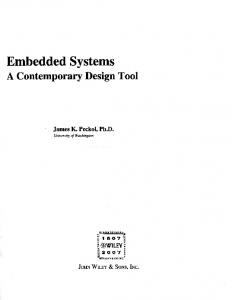
demonstrate the refinement steps, show the problem diagrams and show what the verification theorem should look like. However, in earlier work we have proven a description of this example with PVS [3]. Due to lack of space our example covers not all aspects of the modelling method suggested. In the first place, we focus here on decomposition. The elaboration of verification theorems requires more formal involvement and space, which also holds for the use of patterns. The example is a small PLC-controlled Lego-plant that sorts yellow and blue blocks according to their colour (see figure 2). A number of blocks is in a queue. When the belt is moving the first block of the queue moves to the belt. At the scanner the colour of a block can be detected. A block moves further on into the sorter. The sorter consists of two fork-like arms, each driven by its own motor and equipped by an angle-sensor that can be used to check whether the sorter arm has made a full rotation. The task of the control program is in principle simple: the belt has to move unless there is a block being sorted and at the same time a new block at the scanner. If there is a block in the sorter it has to be moved to the correct side.

The system: A control application Property tree

Physical environment E

Control machine C

P D1 P1

P3

P2

P4

D2

D4

Actuator

D5

Sensor

Programmable device (e.g. a PLC)

D3 Program

P5

Motor C

Rotation C

Light

Queue Conveyer Belt

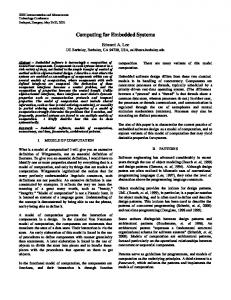
Figure 1: Stepwise decomposition of the environment model

Motor B

and the correctness proof. P is a property of desired behavior D of the environment. D is decomposed into Di and and Pi is a property of Di .

Rotation B Scanner

Motor A

Figure 2: Top view on the Lego plant

Describing all possible behaviour of the environment typically ends up in models that are too large for computer aided analysis. Therefore, a relevant aspect here is that we restrict the description to the desired behaviour (and the error cases we do want to consider). Patterns. Another relevant ingredient of our method is the use of problem and modelling patterns, following the idea of problem frames introduced by Jackson [1, 2]. Using patterns gives (at least) two advantages: first, it makes a decomposition argument more transparent, because we can use some form of standard argument, and, second, it makes the decomposition steps more reliable, because we make use of well-proven solution fragments. To make the idea of problem frames useful we need a library of identified patterns with modelling solutions.

The Lego plant is controlled by a programmable logic controller (PLC), a P8 from Nyquist. The control program structure is written in the language Sequential Function Charts (Petri-net like), extended by the low level language Instruction Lists. The first design step is to state explicitly which fragment of the system is modelled, which is, due to the size, the whole system here. Additionally, we start with some assumptions: E.g., there are only blue and yellow blocks in the queue, no other colour. We start with a description of the system by a problem diagram in figure 3, which corresponds to an architectural description. We have a Requirement R0 and the interface description a. In the verification theorem the requirement R0 represents the desired property. The interface description a contains the phenomena that should occur in both 3 An example models, the one of the plant and the one of the machine. In this section we will illustrate our ideas by an exam- Informally, we have R0 : All blocks will be sorted evenple. Our example is not worked out in detail, we only tually by the plant. 2

R0

Plant

a

The interface descriptions (for the example here, informally) are:

MACHINE

a1: a2:

Figure 3: Problem diagram of the Lego plant and the Machine (Control)

a3:

The verification theorem in its first version is: Plant ∧ Machine =⇒ R0 Because at this level of abstraction we do not have enough details for a meaningful description we continue with the first refinement. Figure 4 contains the first refinement step.

p1: p2: p3:

The machine switches the belt on and off. The scanner sends 3 values to the machine, blue, yellow and nothing. The sorter sends the angle positions of the arms to the machine; the machine switches each sorter arm on and off. The first block of the queue moves to the belt, or nothing moves to the belt. The scanner detects whether there is either nothing or a yellow block or a blue one at the scanner position. If a block is at the end of the belt and the belt is moving (and the sorter is idle), then the block moves to the sorter.

QUEUE

The verification theorem at this stage has the form Queue ∧ Belt ∧ Scanner ∧ Sorter ∧ Machine ∧ NatuBELT ral Laws =⇒ R1 a1 p2 where all elements should be filled in by a description R1 a2 p3 that should formalize the informal description above. MACHINE SCANNER r2 Note that in the verification theorem we do not have a3 explicit interfaces. The composition is done by the logiSORTER cal ∧, and all phenomena taking place on the interfaces should be part of the component descriptions sharing Figure 4: Refined problem diagram of the Lego plant and the the interface. Machine (Control) The Natural Laws typically contain facts as: If the belt is not moving a block on the belt remains in its position. or A R1 = All blocks in the Queue are eventually moved by the block does not change its colour. r1

p1

Sorter to the correct side. r1: Eventually all blocks of the Queue are gone. r2: Eventually all blocks are on the correct sides of the Sorter.

QUEUE p21

The informal component description is:

r1

Queue: Stores unsorted yellow and blue blocks and moves a block on the Belt. Belt: Transports blocks alongside the Scanner, to the Sorter. The speed of the belt is either v or 0. The block is present in front of the Scanner for a minimum time of t = vl seconds, where v is the speed of the belt (in meters per second) and l is the length of a block (in meters). Scanner: Scans the part of the path through which a block is transported from the Queue to the Sorter, recognizes blue, yellow and absence of blocks. Sorter: Sorts a block outside the plant on the appropriate side by rotating only one of the two arms depending of the block’s colour. After a full rotation a block is gone and the sorter is idle again. Machine: The Machine switches the Belt on if there is no block at the Scanner. The Machine switches the Belt on if the Sorter is idle. It switches the Belt off, if there is a block in the Sorter and a block at the Scanner. The Machine moves the Sorter arms according to the colour of the block in the Sorter. A Sorter arm is moved only for one full rotation. The Machine continuously receives one of three possible values from the Scanner.

R2

BELT'

p24

MOTOR A

p22

MACHINE

a22

p23 r2

a21

SCANNER p27 p25

ARMa22 B

p26

ARM C

SORTER'

p28 p29 p30

MOTOR B

a231

ROTATION B MOTOR C ROTATION C

a232 a233 a234

Figure 5: Second refined problem diagram of the Lego plant and the Machine (Control)

We perform a second refinement step, introducing the actuators (motors), and the sensors (scanner, anglesensor). R2 remains unchanged wrt R1 , and also r1 and r2 remain the same. 3

The component descriptions remain almost the same. The extensions with the additional elements are more or less obvious, and we omit them due to lack of space. The interface descriptions, again informally, are:

in general. We can have an architectural, a fuctional or a process-oriented decomposition as in [5], where the method suggested here has been performed in detail. The second source for patterns comes from assumptions a21: The machine switches Motor A on and off. in PLC modelling. Roughly, the assumptions concern a22: The scanner sends 3 values to the machine, blue, the relative times of the PLC scan-cycle in comparison yellow and nothing. to the real-time requirements of the environment. This a231: The machine switches Motor B on and off. allows for different modelling decisions for the control, a232: The machine gets one of 16 different values for the as instantaneous, periodic or lazy reaction, [4]. angle position of Arm B. Control problem frames. The idea of problem frames a233: The machine switches Motor C on and off. a234: The machine gets one of 16 different values for the (rather than solution patterns) was introduced by Jackson [1, 2] as a means to identify reusable problem strucangle position of Arm C. p21: The first block of the queue moves to the belt, or tures in different problem domains. In our example we nothing moves to the belt. used a simple control frame, as also in Jackson’s sluice p22: The scanner detects whether there is either noth- control. Specific issues to be addressed for frames are: ing or a yellow block or a blue one at the scanner (1) The compositionality of problem (solution) frames position. (2) The robustness of decomposition trees under small p23: If a block is at the end of the belt and the belt is changes in properties and/or environments (3) Systemmoving (and the sorter is idle), then the block moves atic analysis of environment assumptions and conseto the sorter. quences of their failure to hold. p24: Motor A moves the Belt’. Model justification. Another research question is if p25: A block in the Sorter’ lies also on Arm B. informal engineering argumentation (physical, graphip26: A block in the Sorter’ lies also on Arm C. cal, ...) can be combined with formal reasoning. We p27: Motor B moves Arm B. p28: Rotation B senses the angle position of Arm B. believe that the decomposition process should provide p29: Motor C moves Arm C. the justification of the accuracy of the model wrt the p30: Rotation B senses the angle position of Arm B. required property. The decomposition process may be Analogously, the verification theorem now includes spec- constrained by the education of the plant engineer and available formal languages. Visual representations of ifications (descriptions) of all components. So far, we have sketched what a decomposition could the formal decomposition that are understandable to the look like and roughly indicated the form of the verifi- plant engineer may help. cation theorem(s). What could not be covered here is Acknowledgment. This paper benefited from extenthe explicit statement of the (formal) models, verifica- sive discussions with Michael Jackson. tion performed, and patterns used for decomposition. Note, that [3] contains an earlier version of this example where descriptions (models) are both in Uppaal and References PVS, which were also used for verification.

4

[1] M.A. Jackson. Software Requirements and Specifications: A lexicon of practice, principles and prejudices. AddisonWesley, 1995.

Discussion and conclusions

[2] M.A. Jackson. Problem Frames: Analysing and Struc-

Our modelling method progresses from a top-level unturing Software Development Problems. Addison-Wesley, derstanding of the system in its environment into more 2000. detailed understanding, decomposing the environment [3] J. Kratz. A case study in PLC control: two ways of model and its desired properties in parallel. We stop deverifying PLC control software for a lego plant, 1999. composing when we reach environment phenomena that can be observed or controlled by the control machine. [4] A. Mader. A classification of PLC models and applications. In 5th Int. Workshop on Discrete Event Systems At that level, we have obtained a correct specification of (WODES) – Discrete Event Systems, Analysis and Conthe controller. We have applied this method on several trol, pages 239–247. Kluwer Academic Publishers, 2000. cases, including the one discussed in this paper [3, 5]). Many research questions remain, some of which we men- [5] A. Mader, E. Brinksma, H. Wupper, and N. Bauer. Design of a PLC control program for a batch plant - VHS tion here. case study 1. European Journal of Control, 7(4):416–439, Patterns. We can identify two sources for patterns: 2001. the first is the decomposition of physical environments 4