A Modified Mountain Clustering Algorithm based on Hill Valley Function

916

JOURNAL OF NETWORKS, VOL. 6, NO. 6, JUNE 2011

A Modified Mountain Clustering Algorithm based on Hill Valley Function Junnian Wang* and Dunshun Liu Hunan Universities Key Laboratory of Knowledge Processing and Networked Manufacturing, Hunan University of Science and Technology, Xiangtan, 411201, China [email protected], [email protected] Chao Liu School of Information and Electrical Engineering, Hunan University of Science and Technology, Xiangtan, 411201, China Email: [email protected]

Abstract—A modified mountain clustering algorithm based on the hill valley function is proposed. Firstly, the mountain function is constructed on the data space, with estimating the parameter by a correlation self-comparison method, and database’s mountain function values are computed. Secondly, the hill valley function is introduced to partition the data distributed on each peak. If the hill valley function’ value of two datum equal to 0, it means these two datum are on the same mountain and belong to the same cluster, otherwise they are not. Finally, the data in a cluster with maximum mountain function value is selected as the cluster centre of this cluster. The testing of four databases indicate that the proposed clustering algorithm can categorise the data numbers in each cluster and find all the cluster centres exactly, and no need priori parameters and stopping criterion correlating to the database. Index Terms—data cluster, hill valley function, mountain clustering method, correlation self-comparison method

I.

INTRODUCTION

Clustering analysis is the process of grouping together similar data patterns into a number of clusters. The main objective of clustering analysis is to classify unlabeled patterns into a number of clusters according to some criteria. It requires the patterns in one cluster should be similar to each other and different from patterns in other clusters. Conventional clustering algorithms, such as k-means and fuzzy c-means, most have the disadvantages of the clustering results correlate with the parameters of algorithm, the initial cluster centers, the input sequence of data patterns, and more required prior parameters. Because the kernel based clustering algorithms can conquer some disadvantages of conventional clustering methods, they are widely used in many applications[1,2,3]. At present, there are two ways of implementing kernel based methods to clustering process: one way is to transform the data space into a high*Corresponding author: Tel:+86-731-58290133.

© 2011 ACADEMY PUBLISHER doi:10.4304/jnw.6.6.916-922

dimensional feature space where the inner products can be represented by a Mercer kernel function defined on the data space. The other way is to find a kernel density estimate on the data space and then search the modes of the estimated density. The mean shift clustering method[4,5] and the mountain clustering method[6] are two simple techniques that can be used to find the modes of a kernel density estimate. The mountain clustering method, proposed by Yager and Filev[5], is a simple and effective algorithm as an approximate clustering. This method is usually used to obtain the initial cluster centers of some advanced clustering algorithms such as k-means and fuzzy c-means. It can also be used alone as a stand method for approximating estimate for clustering centers. Because the mountain method is computed in the amount of computation growing exponentially with the increase in the dimensionality of the data, Chiu[7] modified it by considering the mountain function on the data points instead of the grid nodes. Then the ‘cognition only’ particle swarm optimization algorithm is used in [8,9] to find the clustering centers of mountain clustering. These modified methods can reduce the amount of computation certainly. However, the performance of these mountain methods depends heavily on the mountain function parameter α, the revised mountain function parameter γ, and the stopping criterion δ. Yang and Wu[10] modified the mountain method and proposed a modified mountain clustering algorithm(M-Mountain). The MMountain algorithm can automatically estimate the mountain parameter α with the structure of the data set based on the correlation self-comparison method. And this algorithm can also reduce the effect of parameter γ to the clustering result by a mountain shape correlative parameter β instead of γ. But the stopping criterion of M-Mountain algorithm depends on the maximum of a validity index which is obtained by running the clustering algorithm many times, but can not stop automatically and completely eliminate the effects of parameter γ on the clustering results. On the other hand , because this clustering can not identify the data numbers of a cluster and a data pattern belongs to

JOURNAL OF NETWORKS, VOL. 6, NO. 6, JUNE 2011

917

which cluster, it is difficult to appraise the clustering algorithm by conventional validation criteria(It requires the patterns in one cluster should be similar to each other and different from patterns in other clusters). In this paper, a hill valley function is introduced to MMountain clustering algorithm, and a hill valley function based mountain (H-Mountain) clustering algorithm is proposed. In the H-Mountain algorithm, Firstly, the mountain function is constructed on the data space with estimating the parameter α by a correlation self-comparison method, and then the hill valley function is introduced to partition the data distributed on each peak. Finally, the data in a cluster with maximum mountain function value is selected as the clustering centre of this cluster. Because it doesn’t need to destroy the mountain peaks subsequently, the effects of parameter γ are eliminated completely in the new algorithm. In addition, H-Mountain algorithm stops running automatically when the data distributed on every peak is parted by hill valley function, so no need additional stopping criterion and can be appraised using conventional clustering algorithm validation criteria. II.

n

-α d ( x j , Ni )

, i = 1,2,...

* k −1

i

i

* k −1

)⋅e

− γ d ( N k*−1 , Ni )

and Ni are in direct proportion with

M k −1 ( N1* ) ,but inversely proportional to the identified cluster

(1)

j =1

Where, xj (j=1, …, n) is the jth pattern point, α is a 2 positive constant according to the data set. d ( x j , N i ) = x j − Ni . The formula (1) indicates that every pattern point xj contributes the high value of the mountain function, and the contribution is inversing to the distance between the pattern point xj and the grid point Ni. The mountain function value, M(Ni), tend to higher while the number of patterns close by Ni increases, and the mountain function value tend to play down while the number of patterns close by Ni decreases. So the mountain function can be regarded as an index of data patterns density. The parameter α is important in mountain cluster method. It not only decides the high value but also

© 2011 ACADEMY PUBLISHER

i

To find other cluster centers, we must eliminate the effects of the cluster center that have already been identified. To achieve this, a value inversely proportional to the distance of the grid point from the found centers is subtracted from the previous mountain function. This process is carried out using the equation: M k ( N i ) = M k −1 ( N i ) − M k −1 ( N k*−1 ) ⋅ e− γ d ( N , N ) (3) Where M k −1 ( N k*−1 ) = max{M k −1 ( N i )} (4) M k −1 ( N

PREVIOUS WORKS

A. The Mountain Method The original mountain clustering method (O-Mountain), proposed by Yager and Filev [1] , is a simple and effective method for approximate estimation of the cluster centers based on the concept of a density function. The original mountain method, involves the following three steps: The first step is to form a grid on the data space. All the grid points of the data space, denoted by { Ni }(i=1,2,…), shall initially be considered as possible cluster centers. The clustering performance of the mountain method strongly depends on the grid resolution, with finer grids giving better performance. As the grid resolution is increased, however, the method becomes computationally expensive. In the general way, the grid is formed equably. But the literature [1] did not claim it and that the non-uniform grid is used to express the prior knowledge of the patterns distribution. The second step is the construction of the mountain function which denotes the data patterns density. The mountain function of grid point Ni is given by M 1 ( Ni ) = ∑ e

the smooth of mountain function. So the clustering results are very sensitive to the selection of the parameter α. The third step involves the identification of cluster centers by subsequent destruction of the mountain peaks. In this step, the grid point which has the largest mountain function value is selected as the first cluster center (one of them is selected as the first cluster center if there are multi highest mountain peaks). Let N1* is the first cluster center, it is found with M 1 ( N1* ) = max{M 1 ( N i )} (2)

center N1* . The new mountain function value M k ( N1* ) =0, and then the grid point that has the largest value of new mountain function M k ( N i ) is selected as the second cluster center. The identification process is continued until the enough cluster centers are identified. The clustering performance of the original mountain method strongly depends on the grid resolution, with finer grids giving better performance. As the grid resolution is increased, however, the method becomes computationally expensive. Moreover, the original mountain method becomes computationally inefficient when applied to high dimension data because the number of grid points required increases exponentially with the dimension of data. Chiu[7] suggested an improved version of mountain method, referred to as the subtractive method, in which each data point is considered as a potential cluster center and the mountain function is calculated on the data points rather than grid points. The mountain function at a data point xi is defined as n

M 1 ( xi ) = ∑ e

-α d ( x j , xi )

, i = 1, 2,...

(5)

j =1

The revised mountain function which is used to find subsequent cluster centers is defined as M k ( xi ) = M k −1 ( xi ) − M k −1 ( N k*−1 ) ⋅ e −γ d ( N , x ) (6) * k −1

i

B. The correlation self-comparison method In order to reduce the computation and the effects of the parameter α, Yang and Wu[10] proposed a modified mountain clustering algorithm(M-Mountain). In this algorithm, they defined a modified mountain function on the data space as follows n

P1 ( xi ) = ∑ e j =1

- m β d ( xi , x j )

, i = 1, 2,..., n

(7)

918

JOURNAL OF NETWORKS, VOL. 6, NO. 6, JUNE 2011

Where ⎛∑

β =⎜ ⎜ ⎝

n j =1

−1

xj − x ⎞ ⎟ , ⎟ n ⎠

x=

∑

n j =1

xj

(8)

n

The role of the parameter β is a normalization term which normalizes dissimilarity measure d(xi, xj). Using the parameter m in the modified mountain function P1(xi) is an important step because the m in (7) will become the only parameter of the data set by taking β as the inverse of the dispersion of the data set. Then the correlation selfcomparison is introduced to estimate the parameter β. In order to execute the correlation self-comparison procedure as a computer program, the modified mountain function (7) is rewritten as n

P1m0 ( xi ) = ∑ e

- m0 β d ( xi , x j )

(9)

j =1 n

P1ml ( xi ) = ∑ e

- ml β d ( xi , x j )

(10)

j =1

Where, m0=1，ml=5l (l=1,2,3,…). The correlation selfcomparison procedure can be summarized as follows:

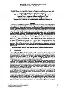
whose fitness is lesser than the minimal fitness of ep and eq, otherwise the points ep and eq don’t belong to the same peak and HV(ep, eq) returns 1. The interior point iinterior can be calculated as[8] iinterior = e p + (eq − e p ) ⋅ samples[ j ] (11) Where a sample array is used and j is jth entry in the array. The upper boundary j is the length of the samples which is referred as sample rate (SR). An one-dimensional (1D) hill valley function is described in Fig.1. For the points e1 and e2, the fitness of the interior points i1~i3 are all greater than the minimal fitness of e1 and e2 and there are no interior point whose fitness is less than the two points. Then it can be claimed that the points e1 and e2 belong to the same peak. For the point e3 and e4, in contrast, there is an interior point i5 whose fitness is less than the fitness of points e3 and e4, and it can be decided that the two points e3 and e4 do not belong to the same peak of the multimodal function. 3

2.6

i 2 i3

2.4

Set l=1 and w=0.99; m Calculate the correlation of the value of P1 ( l −1) ( xi ) and ml 1

P ( xi ) ; IF the correlation is greater than or equal to the specified w, m THEN choose P1 ( l −1) ( xi ) to be the modified function; ELSE l=l+1 and GOTO step 2.

e4

i4

2.8

2.2

i1

e2

2

i6

e3

e1

1.8 1.6 1.4

0.2

i5 0.3

0.4

0.5

0.6

0.7

0.8

0.9

1

Figure1. Sketch map of 1D hill valley function

After the mountain function approximating the data set density shape is obtained by using the correlation selfcomparison procedure, the cluster centers are selected by destroying the mountain gradually. In order to reduce the effects of the revised function parameter γ to the clustering result, γ is replaced by the parameter β. III.

HILL VALLEY FUNCTION BASED MOUNTAIN CLUSTERING ALGORITHM

In the modified mountain function clustering algorithm (M-Mountain) proposed by Yang and Wu[10], the effects of the parameter γ to the clustering result are reduced more or less, but not be eliminated completely. Moreover, the clustering result of this modified mountain clustering algorithm depends heavily on the previous setting stopping criteria. In this section, a hill valley function based mountain clustering algorithm (H-Mountain) is proposed in order to conquer the limitations of M-Mountain. A. Hill valley function The hill valley function proposed by Usrsem[12] provides a method to determine whether two points of a searching space belong to the same peak of multimodal function or not. Let ep and eq are two arbitrary points in a searching space, and HV(ep, eq) is the hill valley function of ep and eq. The points ep and eq belong to the same peak and the hill valley function HV(ep, eq) generally returns 0, if there are no interior iinterior between the points ep and eq

© 2011 ACADEMY PUBLISHER

The procedure of calculating hill valley function value of points ep and eq are presented as follows: Hillvalley(ep , eq , samples) Hillvalley=0; minfit=min(fitness(ep), fitness(eq)); for j=1:length(samples) Calculate the point iinterior on the line between the points ep and eq; If minfit>fitness(iinterior) Hillvalley=1; endif endfor

B. H-Mountain clustering algorithm The first two steps of H-Mountain clustering are similar to the modified mountain clustering algorithm which is proposed by Yang and Wu[10]. In our H-Mountain clustering, the mountain function approximating the data set density shape is obtained by using the correlation selfcomparison procedure. Then the hill valley function is introduced to partition the data distributed on each peak, and the data in a cluster with maximum mountain function value is selected as the clustering centre of this cluster. The pseudocodes of the H-Mountain clustering algorithm are presented as follows: Initialization l=1; w=0.99; samples=[0:0.1:1];

JOURNAL OF NETWORKS, VOL. 6, NO. 6, JUNE 2011

Regarding this algorithm, some points are remarked as follows: 1) Initialization: Main initial parameters are the threshold w and sample vector samples. These two parameters are insensitive and usually w=0.99 and samples=[0:0.1:1]. 2) Construction of mountain function: The mountain function is constructed according to formula (9) and (10) . 3) Estimation of the parameter ml : using correlation self-comparison procedure to estimate the parameter ml. 4) Mountain function value of the patterns: Choose m P1 ( xi ) to be the mountain function and compute the mountain function of data pattern xi (i=1,…, n). 5) The hill valley function value. The hill valley function value of patterns xi、xj (i=1, …, Np，j=1, …, Np， i≠j), Hillvalley(xi,xj), is the hill valley function value of points Di(xi, P1m ( xi ) ) and Di(xj, P1m ( x j ) ). The patterns xi and xj belong to a cluster when Hillvalley (xi,xj)=1. 6) The cluster center of each cluster: selecting a pattern which mountain function value is maximal in the cluster { Nk } as the center of this cluster, calculating the mean of patterns belong to { Nk } as the center of it. In the experiment of this paper, we adopt the first method to obtain the center of cluster { Nk }. 7) Stopping criterion. The algorithm stops running when all patterns which belong to same peaks are transferred to same cluster.

samples=[0:0.1:1] in clustering algorithm.

M-Mountain

and

H-Mountain

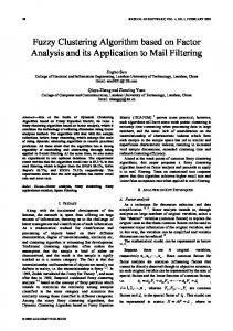
A. 1-D data set A normal mixture data set, named database1, is generated randomly according to literature [10]. The mixed distributions include N(0, 0.8), N(3, 0.5), N(6, 0.8), N(9, 0.5) and N(12, 0.8). The data set of database1 contains 250 data points. Under the threshold w=0.99, m=10 is chosen, and the H-Mountain clustering result is shown on figure 2. Where the asterisks “*” represents the data points, “●” represents the mountain function constructed on the data points, and “○” represents the peak of the mountain function. They are the mountain function of the cluster centers. We compare the performance of the proposed HMountain clustering algorithm with the O-Mountain and M-Mountain clustering algorithm according to the database1. The clustering results are shown in table 1. 30 25 p(x)

Hill_valley=1; Construction of mountain function on the data space; Obtain the mountain function parameter ml using correlation self-comparison procedure; Compute the mountain function values of database; i=1; k=0; while i≤length(database)-1 k= k+1； Create a new cluster { Nk }; Copy the data xi to the cluster { Nk }； j=i+1; while j≤length(database) Calculate the hill valley function value Hillvalley(xi, xj); if Hillvalley(xi , xj)=0 Copy the data xj to the cluster { Nk }; Delete data xj from database； j=j-1; endif j=j+1; endwhile i=i+1; endwhile Find the cluster center of each cluster { Nk }.

919

20 15 10 5 0

6 8 10 12 x Figure2. database1 and it’s H-Mountain clustering results

TABLE I.

0

2

4

COMPARISON OF THE THREE ALGORITHMS TO DATABASE1

( l −1)

l

IV.

l

EXPERIMENTAL RESULTS

Three patterns sets were used to evaluate the proposed clustering algorithm and comparison was performed between O-Mountain, M-Mountain, K-means, and the proposed H-Mountain clustering algorithm. Where the stopping criteria of O-mountain, and w=0.99,

© 2011 ACADEMY PUBLISHER

algorithm Center number 1 2 3 4 5 6 7

H-Mountain ⁄ 0.2 3.0 5.3 8.9 12.0

H-Mountain/ O-Mountain γ=β 3.0 11.9 8.8 -0.3

γ=5β 3.0 8.9 12.0 0 5.8 12.1 -2

From table 1, it can be observed that, the proposed HMountain clustering algorithm find the five cluster centers of database1 accurately without prior data based parameters. Although the M-Mountain clustering algorithm can obtain the clustering results according to the parameter γ=β, it is not so well, for there only find four clustering centers of five clusters in the database1. But O-Mountain method depends not only on the parameters α and γ, but also the stopping criteria. B. 2-D data set A 2 dimensional data set database2, contains 291 data points and 3 clusters, is created randomly. Using the proposed H-Mountain clustering, under the choose of m=10, the clustering result of database2 is shown on figure 3 a)and b). Where symbol “○” represents the data points,

920

JOURNAL OF NETWORKS, VOL. 6, NO. 6, JUNE 2011

“☆”represents the found cluster centers, “*”represents the mountain function constructed on the data space. We compare the performance of the proposed HMountain clustering algorithm with the O-Mountain and MMountain clustering algorithm according to the database2. The clustering results are shown in table 2. From table 2, it can be observed that, the clustering results of H-Mountain clustering algorithm, be similar to M-Mountain under δ=0.5. While the clustering results of O-Mountain have great dissimilarity under different value of parameter γ.

classic test data sets – Iris plant data set, the data set contains three clusters of 150 four-dimensional sample vector. The proposed H-Mountain clustering algorithm is examined using the above four patterns sets and is compared with the conventional k-means clustering algorithm. Table 3 provides a comparison of two algorithms in the average of running 20 times. Where Intra and Inter represent two widely validation criterias of clustering algorithm respectively, named compactness and separation. The variance of patterns in a cluster gives an indication of compactness and the Euclidean distance between cluster centers gives an indication of cluster separation. Intra and Inter were computed as follows [13] 1 K Intra= ∑ ∑ x - N k* n k =1 ∀x∈Nk*

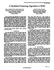
C. 3-D data set 3 dimensional data set database3, contains 600 data points and 11 clusters, is created randomly and shown on figure 4a). Using H-Mountain clustering, under the choose of m=30, the cluster centers of database3 are shown on figure 4 b). D. 4-D data set The fourth test sample data sets to be choosen is a

Inter = min{ N k* − N kk* }, ∀k = 1,L , K − 1 , kk = k + 1,L , K

1

60 p(x,y)

0.8

y

0.6

20

0.4 0.2 0

40

0.8

0

0.5 x

0.6

0.4 y

1

0.2

0.2

0.4 x

b). The mountain function of database2

a) . Distribution of database2 Figure3. database3 and the clustering of H-Mountain TABLE II. algorithm Center number 1 2 3 4 5 6 7

© 2011 ACADEMY PUBLISHER

COMPARISON OF THE THREE ALGORITHMS TO DATABASE2 H-Mountain

∕

H-Mountain/ O-Mountain γ=β

(0.6333, 0.1995) (0.6333, 0.1995) (0.1993, 0.6005) (0.8046, 0.8074) (0.8102, 0.7872) (0.1594, 0.5968) ∕ ∕ ∕ ∕ ∕ ∕ ∕ ∕ ∕ ∕

γ=5β

γ=8β

(0.6333, 0.1995) (0.1993, 0.6005) (0.8102, 0.7872) (0.7798, 0.7684) ∕ ∕ ∕ ∕

(0.6333, 0.1995) (0.1993, 0.6005) (0.8102, 0.7872) (0.5518, 0.2124) (0.0907, 0.4743) (0.6719, 0.8510) (0.6160, 0.9924) (0.0763, 0.4600)

0.6

0.8

JOURNAL OF NETWORKS, VOL. 6, NO. 6, JUNE 2011

921

4

4

z

6

z

6

2

2

0

0 6

4

2

2 0 0 y x a) Distribution of database3

4

6

6

4

2 y

0

0

2 x

4

6

b) the cluster centers of database3

Figure 4 database3 and the clustering analysis of H-Mountain

TABLE III.

THE COMPARISON OF H-MOUNTAIN AND K-MEANS

Priori cluster Obtained cluster Intra center numbers center numbers H-Mountain 5 0.0154 ∕ database1 K-means 5 5 1.337 H-Mountain 3 7.936E-04 ∕ Database2 K-means 3 3 0.0156 H-Mountain 11 0.0094 ∕ Database3 K-means 11 11 0.887 M-means 3 0.0851 ∕ Iris plant data set K-means 3 3 0.887 Data set

algorithm

From table 3, it can be observed that the proposed HMountain clustering algorithm obtained all cluster centers and the data points belong to each cluster without prior cluster center number. While the K-means algorithm needs to give the number of cluster centers in prior. When considering the compactness and separation of the two clustering, although the difference of two algorithms in Inter were not too great, but the Intra were obviously different. It was said that the H-Mountain clustering algorithm found clusters large separation than the k-means algorithm. V.

CONCLUSION

A modified mountain clustering algorithm, based on hill valley function, is proposed in this paper. In the proposed algorithm, the mountain function is constructed on the data space, with estimating the parameter by a correlation selfcomparison method. Then the hill valley function is introduced to partition the data distributed on each peak. And finally, the data in a cluster with maximum mountain function value is selected as the clustering centre of this cluster. Comparing with the existed mountain clustering algorithm and its modified algorithm, the proposed algorithm can obtain the cluster centre numbers, cluster centres and the data patterns belong to each cluster centres automatically and accurately. It conquered the disadvantages of existed mountain clustering algorithms, such as the clustering results depend on priori parameters and stopping criteria. It is a self adapting clustering algorithm. Comparing

© 2011 ACADEMY PUBLISHER

Inter 2.266 4.519 0.591 0.171 2.802 3.302 3.374 3.302

with conventional k-means clustering algorithm, the HMountain clustering algorithm obtained all cluster centers and the data points belong to each cluster accurately without prior cluster center number, and the clustering results are obviously better than k-means. ACKNOLEDGMENT

This work was supported by National Natural Science Foundation of China (No. 60974048, 50774032), Hunan Provincial Natural Science Foundation of China （No.08JJ3127 ）and the planned science and technology project of Hunan province(No.2009CK3073). REFERENCES [1] [2] [3] [4] [5]

F. Camastra, A. Verri. A novel kernel method for clustering[J]. IEEE Trans. Pattern Anal. Mach, 2005, 27(5): 801-805. L. Angelini, D. Marinazzo, M. Pellicoro, S. Stramaglia. Kernel method for clustering based on optimal target vector [J]. Physics Letters A, 2006, 357 (6) : 413–416. M. Girolami. Mercer kernel based clustering in feature space[J]. IEEE Trans. Neural Networks, 2002, 13(3): 780784. K. L. Wu, M. S. Yang. Mean shift-based clustering[J]. Pattern Recognition, 2007, 40(2): 3035-3052. Y. Cheng. Mean shift, mode seeking, and clustering[J]. IEEE Trans. Pattern Anal. Mach, 1995,17(8): 790-799.

922

[6] [7] [8]

[9] [10] [11] [12] [13]

JOURNAL OF NETWORKS, VOL. 6, NO. 6, JUNE 2011

R. R.Yager, D. P. Filev. Approximate clustering via the mountain method [J]. IEEE Transactions on Systems, Man, and Cybernetics, 1994, 24(8): 1279-1284. S. L. Chiu. Fuzzy model identification based on cluster estimation. Journal of Intelligent And Fuzzy Systems, 1994, 2(3):267-278. H.Y. Shen, X.Q. Peng, J.N. Wang, Z.K. Hu. A Mountain Clustering Based on Improved PSO Algorithm[A]. First International Conference of Advances in Natural Computation[C], Changsha, China, 2005: 477-481. H.Y. Shen, X.Q. Peng, J.N. Wang. Quick mountain clustering based on improved PSO algorithm[J]. Journal of Systems Engineering, 2006, 22(3): 333-336. M. S. Yang, K. L. Wu. A modified mountain clustering algorithm[J]. Pattern Analysis and Applications, 2005, 26(8):125-138. J. Zhang, D.S. Huang, T.M. Lok, M.R. Lyu. A novel adaptive sequential niche technique for multimodal function optimization[J]. Neurocomputing, 2006, 69(12): 2396-2401. R.K. Ursem. Multinational evolutionary algorithms[A]. Proceedings of Congress of Evolutionary Computation(C), Washington, DC, USA, 1999: 1633–1640. Mahamed G. H. Omran. Particle swarm optimization method for pattern recognition and image processing [D]. University of Pretoria, S. Africa, 2005.

© 2011 ACADEMY PUBLISHER

Junnian Wang received his M.S. degree in radio physics from Lanzhou University, Lanzhou, P.R. China, in 2000 and the Ph.D. degree in control theory and control engineering from Central South University, Changsha, P.R. China, in 2006. He is currently a professor of the Hunan University of Science and Technology. His current research interests include optimization algorithm, data mining and intelligent control. Deshun Liu received his M.S. degree in mechanical engineering from China University Ming and Technology, Xuzhou, P.R. China, in 1985 and the Ph.D. degree in control theory and control engineering from Central South University, Changsha, P.R. China,. He is currently a professor of the Hunan University of Science and Technology. His current research interests include green manufacture, networked manufacture and intelligent control. Chao Liu received his B.S. degree electronic information engineering in from Xi’an University Architecture and Technology, Xi’an, P.R. China, in 2007 and now he is currently working toward the M.S.. degree in control theory and control engineering at Hunan University of Science and Technology. His research interests include data mining and intelligent control..