Haidar Samet1, Abdollah Kavousi-Fard2, Sina Rajabi3 1
2
School of Electrical and Computer Engineering, Shiraz University, Shiraz, Iran Nourabad Mamasani Branch, Islamic Azad University, Nourabad Mamasani, Iran 3 Marvdasht Branch, Islamic Azad University, Marvdasht, Iran
doi:10.15199/48.2015.01.07
A modified teaching-learning based optimization for the location and size of two SVCs to compensate the railway’s voltage drop Abstract. The recent concerns about fossil fuels have made mass transportations such as electric railways more popular than before. Meanwhile, traction loads are generally complex electrical loads that should be managed by the main electric grid when operated by the Railway Company. In this way, static VAr compensators (SVCs) is a precious tool for preserving the power quality of the electric grid in the presence of electric railways. Therefore, this paper discusses the locating of two SVCs in a rail way with modified teaching- learning based optimization (MTLBO). The results are compared with performing the optimization by Particle swarm optimization (PSO) algorithm. Streszczenie. W artykule analizuje się metody optymalizacji położenia i rozmiaru statycznego kompensatora mocy biernej SVCs w sieci trakcyjnej. Do tego celu wykorzystuje się zmodyfikowaną metodę optymalizacji bazującej na algorytmie nauczania/uczenia się MTLBO. Metoda optymalizacji położenia i rozmiaru statycznego kompensatora mocy biernej SVCs w sieci trakcyjnej bazująca na algorytmach uczenia.
Keywords: MTLBO, PSO, SVC, Traction systems, Voltage drop Słowa kluczowe: kompensacja mocy biernej, sieć trakcyjna.
Introduction In recent years, a high number of Traction System configurations have been employed throughout the World. Selection of the proper system depends on the train facility conditions, including commuter rail, freight rail, light rail, train loads, and electric grid power supply [1]. Generally, railway is assumed as an appropriate device for regular mass transportations. It is efficiently energy-saving in comparison to other devices such as automobiles and aircraft. In fact, railway has such great potentiality as to answer global ecological concerns of carbon oxide release if it replaces automobiles or aircraft [2]. The main objective of traction systems is to bring energy to the locomotives as proficiently and frugally as possible [3]. From the electric view, the majority of the main line electrified railway systems work at 25 kV 50/60 Hz. Locomotives get energy from a single phase overhead contact feeder through feed transformer to the public network. At this voltage level, traction systems encounter many complications which are not only damaging to the traction system itself, but also may spread over the supply system, troubling other users in the network. Many of these problems initiate from the load movement [3]. The electric locomotives running on the electrified railroads belong to the single-phase, large power, nonlinear loads [4]. These loads produce noteworthy negative-phase-sequence and harmonic currents in the public power system which distresses the quality of electrical services [5-7]. The opposing results of harmonics in power systems contain overheating of rotating machines, signalling and electronic circuits, overloading of capacitors, interference with communication, overstressing of insulation, metering errors and possible system resonance [8]. In the worst situation, over-voltage is produced and small machines and capacitors are burnt out [9]. Especially, harmonic distortion can cause a higher voltage form factor and henceforth a lower locomotive power output [10]. Still, traction loads can cause flicker once the trains pass from one substation to the other. Forecasting the flicker is occasionally very problematic since its changing depends on the generation pattern, system dynamics, etc. [1]. On the other hand, voltage drop at the connection point of the locomotives to the railway main line is another issue in the 25 kV railways. This problem is usually caused by
passing the lagging reactive current in the inductive components of the overhead system [3], [11]. Correction of the voltage level such that trains function typically, limit both the maximum length of the track section (typically 25 km) and the distance between feeding substations, as shown in Fig.1. Besides, these voltage drops affect the maximum power transmitted by the feeder, concerning a limit in the maximum numbers of locomotives feeding simultaneously [3], [12], [13]. Usually, voltage drop will devastate the power of the electric locomotive when polluting the quality of network harshly. In addition, it will destroy the operating security of local power network when no compensation is done [14].
Fig. 1. Typical feeding arrangement of a railway system [3]
In this paper, studies have been carried out on a 25 kV railway electrification system. Here, the railway system is divided into several electrical sections with the span of 25 km. Longer sections cause an excessive voltage drop (more than 25%) with severe loss of performance to the most distant locomotives [11]. Feeding longer track section is normally probable by installing supplementary substations however it is an affluent procedure. Consequently, it is vital to examine techniques for extending the feasible length of track section more than 25 km. In the railway systems, owing to the regularly changing characteristics of the load, passive equipment cannot regulate the compensating ability to the load needs, wherever over- compensation and under-compensation happen normally [15]. By the utilization of Static VAr Compensators (SVCs), the voltage drops is eliminated. Technically, SVCs are controllable reactive power sources, with controlled or variable capacitors or inductors [16]. It is demonstrated in the literature that a conventional Thyristor Controlled Reactor (TCR) in parallel with a fixed capacitor (FC) can adequately trail the traction load alterations [3].
PRZEGLĄD ELEKTROTECHNICZNY, ISSN 0033-2097, R. 91 NR 1/2015
41
Previous studies have shown that using two SVCs connected to the middle and end of the feeder, can increase the section lengths to 75 km [17, 18]. With regard to what mentioned above, in this paper we have been used two SVCs (TCR/FC) to compensate the voltage drop over the main line of railway’s supply with length equal to 120 km. Modified teaching - learning based optimization (MTLBO) is implemented to optimal locating of the SVCs (their sizes and locations). The results are compared with performing the optimization by Particle swarm optimization (PSO) algorithm. Original TLBO In response to the deficiencies of the traditional optimization algorithms such as requiring derivatives and assumptions in solving the problems, evolutionary algorithms were proposed in the last years as new stochastic methods. The existence of some characteristics such as random nature, low adjusting parameters and no need to derivative made the evolutionary algorithms popular solutions in the short time. Some of the most outstanding evolutionary algorithms can be named as shuffled frog leaping algorithm [19], honey bee mating optimization algorithm [20], particle swarm optimization (PSO) algorithm [21, 22], clonal selection algorithm [23], firefly algorithm [24, 25], etc. While each of these algorithms can be promising techniques for different problems but they suffer mainly from high dependency on their initial parameters. In order to overcome this issue, a new algorithm based on the behaviour of teacher and students in a class was proposed in 2011 called teacher learning-based optimization (TLBO) algorithm. The superiority of TLBO over some of the famous optimization algorithms is demonstrated in [26-27]. TLBO algorithm performs based on two main ideas: 1) students should try to enhance their knowledge toward the teacher knowledge as the best individual in the class (called teacher phase) and 2) students improve their knowledge by interaction with each other and debate (called learner phase). Similar to any other evolutionary algorithm, TLBO starts with generation of a random initial population. The quality of each student is determined according to his/her grades as follows:
X [x 1 , x 2 , x 3 ,..., x N ]
i i i i i (1) where N is the length of the control vector. Now, the above two ideas are employed as the improvisation stages as follows: Teacher phase: In order to simulate this event, all the students should move toward the teacher position. In this regard, the mean value of the students' grades is calculated column-wise (MD). Now, the mean of the students' grads should be moved toward the teacher as follows:
X new X old (X Teacher ,Q T F M D ) M Q [m1 , m 2 , m 3 ,..., m N ]
(2)
where TF is an integer value equal to 1 or 2 and γ is a random value in the range of [0,1]. If Xnew is better than Xold (a student with higher grades) then replace it. Learner phase: As described before, this phase simulates a consultation among the students. This process between the student Xi and student Xj is simulated as follows: For i =1:Nclass (3)
If F ( X i ) F ( X j )
X new,i X old ,i 1 (Xi X j )
If F ( X i ) F ( X j )
X new,i X old ,i 2 (X j Xi )
End if End for
42
where F(X) is the objective function value of the student X ; Also µ1 and µ2 are random values in the range of [0,1]. Modified TLBO (MTLBO) As mentioned previosuly, TLBO is a powerful optimziation algorithm with especial feaceures such as simple concept, easy implementation, little adjusting parameters and high search ability [27-28]. Nevertheless, we propose a new modification method to improve the total search ability of this algorithm in both local and global searches. Here we make use the of croosover and mutation operators to increase the diversity of the popualtion and thus improve the convergence of the TLBO. In this way, for each student (Xs) and in each iteration, three students (Xd1, Xd2, Xd3) are selected such that Xd1 ≠ Xd2 ≠ Xd3 ≠ Xs. Using these three students, a new modified individual is generated as below:
X muted X d (X d X d )
1 2 3 (4) Now by the use of XTeacher, Xmuted and Xs three new modified learners are generated as the follows:
(5)
x muted , j , if 1 2 x mut 1, j x Teacher , j , Else x muted , j , if 3 2 x mut 2, j x s , Else X m ut ,3 X Teacher ( X Teacher X muted )
where 1 , 2 , 3 and ρ are random values in the range of [0,1]. The most suitable individual among Xmut1,j, Xmut2,j, Xmut3 and Xs is chosen as the new improved learner that will replace Xs in the class. The complete flowchart of the proposed MTLBO is depicted in Fig. 2. Particle Swarm Optimization (PSO) PSO is a population based stochastic optimization technique in which the potential solutions (called particles) fly through the search-space by following the current optimum particles. This process is according to the simple mathematical formulae based on the particle’s position and velocity [29]. In every iteration, each particle is updated by following two "best" values. The first one is the best solution which is called p-best. Another "best" value is a global best and called g-best. After finding these two best values, the particle updates its velocity and positions by using following equations: v[ ] = v[ ] + C1 * r * (pbest[ ] - present[ ]) (6) (7)
+ C2 * r * (gbest[ ] - present[ ]) present [ ] = present[ ] + v[ ]
v[ ] is the particle velocity, present[ ] is the current particle (solution); pbest [ ] and gbest[] are defined as stated before. r is a random number between 0 and 1. C1 and C2 are learning factors which usually equal to 2. For using PSO, it’s not necessary that the optimization problem be differentiable because PSO doesn’t use the gradient of the problem [30-32]. Single Track Section To study the voltage drop at the point of locomotives connection to the railway main line, modeling a traction system including several locomotives and the compensator (TCR/FC) is necessary. In this paper, studies are carried out into 27.5kV electrification systems for main line railways (fig.3).The single track section is fed through a single phase step down transformer from the high voltage supply which is modeled by an inductor.
PRZEGLĄD ELEKTROTECHNICZNY, ISSN 0033-2097, R. 91 NR 1/2015
Start
Define the number of students and the termination criterion
Evaluate the objective function for the students Determine the best solution Evaluate the mean value of the class column-wise Modify the students by Eq. 2
Is the new student better than the existing?
No
Reject
Yes Select Xi and Xj Such that Apply Eq. 3 to Xi and Xj
Is the new student better than the existing?
No Reject
Yes For each of the students (Xs) select three students (d1, d2, d3) such that d1 ≠ d2 ≠ d3 ≠ s
By Eq. 4 Xmuted is generated
By Eq. 5 Xmut1,j, Xmut2,j and Xmut3 are generated
Among Xmut1,j, Xmut2,j, Xmut3 and Xs the best one replaces Xs
Is the termination criterion satisfied?
No
Yes Print the best solution
Fig.2. The MTLBO block diagram
Fig.3. Equivalent circuit of a 120 km track section
PRZEGLĄD ELEKTROTECHNICZNY, ISSN 0033-2097, R. 91 NR 1/2015
43
For modeling the system, the whole length of 120 km feeder, is divided into six parts at the end of each part, there is a connection point as a loading point. Each of these parts was modeled by a π-equivalent circuit (fig.3) and each of them each has a longitudinal impedance of (0.169+j0.432)Ω/km at 50 Hz and a shunt capacitance of 0.02µF/km. The movement of locomotive along the railway line has been modeled by considering the time variable line impedance for the first section, as shown in Fig.3. Here, d is the distance of the first locomotive from the feeder section and it changes between 0-20 km. The other locomotives have a constant distance from each other (equal to 20 km). Various locomotive positions distributed along the feeder system can be selected for study.
Fig.4. Simplified model of locomotive for voltage drop studies Table 1. System Parameters Element Vs Rs + Rt Ls + Lt R X C L (each Loco.) I (each Loco.)
Value 27.5 kV 1Ω 0.0271 H 0.169 Ω/km 0.432 Ω/km 0.02 µF/km 0.05 H 68 A
Locomotive Models Depending on the aim of studies (voltage drops or harmonics), two different models are used for locomotive: • A constant current, constant power factor model, including a single diode bridge which is suitable for voltage regulation simulations; and • A full representation for harmonic and dynamic studies. This model is including conventional thyristor converters which are used with delayed firing to control the current in lower speed ranges. However, most of the time these converters operate without any firing delay and speed increasing is achieved by field weakening [11]. A simplified model of locomotive which is used in this paper is shown in Fig.4. In this model, it’s assumed that the transformer is 1:1. The parameters of the railway system using in this paper regarding to one 20 km section are shown in Table.1. Optimizing the location and Capacity of TCR by Using PSO As mentioned later, the aim of this paper is to compensate the voltage drop by using a TCR/FC. In this section, MTLO and PSO are used to optimize the location and size of SVC. For this purpose, MATLAB programming is used where determines the best location and also the least size of SVC so that the voltages of the locomotives’ connection points to the railway main line don’t be less than 25.2 kV. In this optimization the movement of locomotives has been taken to account by supposing that the track sections is divided into six equal sections and the distance between locomotives are constant (equal to 20 km). The distance of the first locomotive from feeding substation is
44
varying between 0-20 km. With running this program, in each step the distance of the first locomotive from feeding substation is increase as 1 km and therefore at the end of running the program we have eighteen different locations. So for each program running, we will obtain 120 different locations for the locomotives. In fact, the output of the program is eighteen different voltages where each of these voltages is the minimum voltage between voltages of four locomotives at each step. The least voltage between these eighteen locomotives’ voltages has been chosen and then by using PSO, the size of SVC has been computed so that this minimum voltage doesn’t be less than 25.2 kV. The steps of this algorithm are as bellow: step1: Input data; step2: Pick random location and capacity for each particle; step3: Run the load flow program and compute all the level of voltages for all locations; step4: Choose the best location; step5: Check all the updated parameters be in the identified ranges; step6: Run the load flow program and compute all the level of voltages for all locations; step7: Update g-best and p-best; step8: Check the termination criteria of the algorithm; step9: If the termination criterion is met, print the results else back to step7.
Here, parameters are the location of two SVCs which are randomly varying between 0-120 km and the size of which has continuously variations in the range of 0-20 MVAr. The termination criteria of the algorithm are the best location and size of SVC so that the minimum voltage of locomotives at the point of connection to the railway main line doesn’t be less than 25.2 kV. The active and reactive powers for each train are assumed to be respectively equal to 2.25 MW and 1 MVAr. Table 2 shows the optimal sizes and locations of two SVCs using MTLBO and PSO. Table 2: Optimal location and sizes of SVC SVC1 SVC2 Method Location(km) Size (kW) Location(km) Size (kW) PSO 3 12651.462 96 7138.9766 MTLBO 61 602.42686 97 6997.0197
Results of 20 times running of MTLBO and PSO programs to obtain the optimum size and location of the SVC are shown in table 3. The minimum voltage among the 4 trains is shown here. Due to the statistical nature of PSO method, we’ve got a different value in each running. Hence in this case MTLBO is more stable than PSO. Table 3: Stability analysis of the MTLBO versus PSO algorithm in the optimization of voltage profile for 20 trails Method Best answer Worst answer Standard deviation PSO 25.6210 25.3437 0.3424 MTLBO 25.6331 25.6331 0.0000
Fig.5. The convergence of MTLBO and PSO
PRZEGLĄD ELEKTROTECHNICZNY, ISSN 0033-2097, R. 91 NR 1/2015
Figure 5 compares the convegence of the two methods. It is evident MTLBO is faster than PSO. Conclusion In this paper, utilizing of two SVCs in case of voltage drop compensation in railway was discussed. In order to solve the problem optimally, a new optimization algorithm called TLBO along with a new modification method was proposed. After introducing some basic concepts of MTLBO and PSO, the location and size of two SVCs over the main line of the railway system was optimized. MTLBO is faster in convergence and more stable than PSO. There is a different answer each time of running PSO but the answer is not changing in case of MTLBO. REFERENCES [1] Bhargava B., Railway Electrification Systems and Configurations. IEEE Power Engineering Society Summer Meeting, (1999), 445-450 [2] Watanabe T., Trend of Railway Technologies and Power Semiconductor Devices, 11th International Symposium on Power Semiconductor Devices and Ics, (1999), 11-18 [3] Celli G., Pilo F., Tennakoon S.B., Voltage Regulation on 25 kV AC Railway Systems by Using Thyristor Switched Capacitor, Ninth International Conference on Harmonics and Quality of Power, (2000) [4] Jianzong M., Mingli W., Shaobing Y., The Application of SVC for the Power Quality Control of Electric Railways. International Conference on Sustainable Power Generation and Supply, (2009) [5] Qun-zhan L., A Study of Parallel Compensation Method in Railway Traction Power Supply Systems, Journal of Southwest Jiaotong University, 2 (1986) [6] Kolar V., Kocman S., Filtration of harmonics in traction transformer substations, positive side effects on the additional harmonics, Przegląd Elektrotechniczny, 87 (2011), nr 12a, 44-46 [7] Xu Q., Zhu Q., Zhang H., Yuan X., A Rigorous Method for Power Quality Evaluation of High-speed Railway Using Electrical Transient Analyzer Program, Przegląd Elektrotechniczny, 88 (2012), nr 11a, 248-252 [8] Barnes R., Wong K.T., Unbalance and Harmonic Studies for the Channel Tunnel Railway System. IEE Proc.-B, I991. Vol. 138. No. 2. [9] QUN-ZHAN L., ZHANG J., Qing-Quan Q., Optimization Design on Series Tuning Filtering and Reactive Compensation Used in Traction Systems. Int. Conf. on Main Line Railway Electrification, (1989), 222-226 [10] Tan P., Loh P., Holmes D., Morrison R., Application of Multilevel Active Power Filtering to a 25 kV Traction System, Australasian Universities Power Engineering Conf., (2002), 1-6 [11] Hu L., Morrison R.E., Young D.J., Comparison of Physical and Digital Modeling Techniques for a Compensated Railway System. Advances in Engineering Software, 19 (1994), 61-67. [12] Kulworaswanichpong T., Goodman C.J., Optimal Area Control of AC Railway Systems via PWM Traction Drives. IEE Proc. Electric Power Applications, 152 (2005), no. 1, 33-40 [13] Tan P.C., Morrison R.E., Holmes D.G., Voltage Form Factor Control and Reactive Power Compensation in a 25kv Electrified Railway System Using a Shunt Active Filter Based on Voltage Detection. 4th IEEE Int. Conf. on Power Electronics and Drive Systems, 2001. [14] Xu X., Chen B., Gan F., Electrical Railway Active Power Filter Research Based on Genetic Algorithms. IEEE Int. Conf. on Control and Automation, 2007.
[15] rahmani S., Alhadad K., A Single Phase Multilevel Hybrid Power Filter for Electrified Railway Applications. IEEE Int. Symp. on Industrial Electronics, 2006. [16] Samet H., Mojallal A., Ghanbari T., Employing Grey System Model for Prediction of Electric Arc Furnace Reactive Power to Improve Compensator Performance, Przegląd Elektrotechniczny, 89 (2013), nr 12, 110-115 [17] Morrison R.E., Warbortun K., Young D.J., The application of shunt compensation on AC railways, IEE Int. Conf. on Electric Railway Systems for a new century, (1987) [18] Morrison R.E., Warbortun K., Hackwell D., The Use of Static Shunt Compensation to Upgrade Existing Electrified Railways. IEE Int. Conf. on main line railway electrification, (1989) [19] Kavousi-Fard A., Akbari-Zadeh M.R., Reliability Enhancement Using Optimal Distribution Feeder Reconfiguration, Neurocomputing, 106 (2013), 1–11 [20] Kavousi-Fard A., Samet H., Multi-objective Performance Management of the Capacitor Allocation Problem in Distributed System Based on Modified HBMO Evolutionary Algorithm, Electric Power and Component systems, 41 (2013), no 13, 1223-1247 [21] Baziar A., Kavousi-Fard A., Consideration Effect of Uncertainty in the Optimal Energy Management of Renewable Micro-Grids including Storage Devices, Renewable Energy, 59 (2013), 158-166 [22] Eslami M., Shareef H., Mohamed A., Khajehzadeh M., Particle Swarm Optimization for Simultaneous Tuning of Static Var Compensator and Power System Stabilizer, Przegląd Elektrotechniczny, 87 (2011), nr 9a, 343-347 [23] Kavousi-Fard A., Niknam T., Optimal Distribution Feeder Reconfiguration for Reliability Improvement Considering Uncertainty, IEEE Trans. on Power Delivery, 29 (2014), no 3, 13441353 [24] Kavousi-Fard A., Samet H., Marzban F., A New Hybrid Modified Firefly Algorithm and Support Vector Regression Model for Accurate Short Term Load Forecasting, Expert Systems With Applications, 41(2014), no 13, 6047–6056 [25] Kavousi-Fard A., Niknam T., Golmaryami M., Short Term Load Forecasting of Distribution Systems by a New Hybrid Modified FA-Backpropagation Method, Journal of Intelligent and Fuzzy systems, 26 (2014), 517-522 [26] Rao R.V., Savsani V.J., Vakharia D.P., Teaching–learningbased optimization: A novel method for constrained mechanical design optimization problems, Computer-Aided Design, 43 (2011), 303-315 [27] Niknam T., Kavousi-Fard A., Baziar A., Multi-objective stochastic distribution feeder reconfiguration problem considering hydrogen and thermal energy production by fuel cell power plants, Energy, 4(2012), no. 1, 563–573 [28] Kavousi-Fard A., A new fuzzy-based feature selection and hybrid TLA–ANN modeling for short-term load forecasting, Journal of Experimental & Theoretical Artificial Intelligence, 25 (2013), no.4, 543-557 [29] Millonas M.M., Swarms, Phase Transitions, and Collective Intelligence. In C. G. Langton. Artificial Life III. Addison Wesley. Reading, MA. 1994. [30] Kenned J., Eberhart R., Particle Swarm Optimization. Proc. IEEE Int. Conf. on Neural Networks, 1995. [31] Kenned J., Eberhart R., Swarm Intelligence, Morgan Kaufmann Publishers, Inc. Sanfrancisco, CA, 2001. [32] Clerc M., The Swarm and the Queen: Towards a determininistic and adaptive particle swarm optimization. In Congress on Evolutionary Computation (CEC99), 1999,1951-1957 Authors: Dr. Haidar Samet, School of Electrical and Computer Engineering, Shiraz University, Shiraz, Iran,
[email protected] Mr. Abdollah Kavousi-Fard,
[email protected] Mr. Sina Rajabi,
[email protected]
PRZEGLĄD ELEKTROTECHNICZNY, ISSN 0033-2097, R. 91 NR 1/2015
45