A Molecular Dynamics Simulation Prototyping Environment - CiteSeerX

MDLab: A Molecular Dynamics Simulation Prototyping Environment

Trevor Cickovski1,Santanu Chatterjee2,Jacob Wenger2, Christopher R. Sweet2,Jes´ us A. Izaguirre2 1 Natural

Sciences Collegium, Eckerd College, 115 Sheen Science C, St. Petersburg, FL 33711, USA 2 Department of Computer Science and Engineering, University of Notre Dame, 384 Fitzpatrick Hall, Notre Dame, IN 46556, USA

Abstract Molecular dynamics (MD) simulation involves solving Newton’s equations of motion for a system of atoms, by calculating forces and updating atomic positions and velocities over a timestep ∆t. Despite the large amount of computing power currently available, the timescale of MD simulations is limited by both the small timestep required for propagation, and the expensive algorithm for computing pairwise forces. These issues are currently addressed through the development of efficient simulation methods, some of which make acceptable approximations and as a result can afford larger timesteps. We present MDLab, a development environment for MD simulations built with Python which facilitates prototyping, testing, and debugging of these methods. MDLab provides constructs which allow the development of propagators, force calculators, and high level sampling protocols that run several instances of molecular dynamics. For computationally demanding sampling protocols which require testing on large biomolecules, MDL includes an interface to the OpenMM libraries of Friedrichs et al. which execute on graphical processing units (GPUs) and achieve considerable speedup over execution on the CPU. As an example of an interesting high level method developed in MDLab, we present a parallel implementation of the On-The-Fly String Method of Maragliano and Vanden-Eijnden. MDLab is available at http://mdlab.sourceforge.net. Key words: molecular dynamics, sampling, Python, scripting, propagation, parallelism, On-The-Fly String Method PACS: 82.20.Wt [Computational modeling; Simulation], 83.10.Mj [Molecular dynamics, Brownian dynamics], 83.10.Rs [Computer simulation of molecular and particle dynamics] Availability: MDL is available open source at http://mdlab.sourceforge.net.

Preprint submitted to Elsevier

10 July 2009

1

Introduction

Molecular dynamics (MD) simulation propagates an atomic system by solving Newton’s equations of motion F = ma, updating atomic positions and velocities over a timestep ∆t. Newtonian dynamics can be characterized more generally by Eq. (1), where U(~x) is the potential energy of the system, ~x is the vector of atomic positions, and ~p is the vector of atomic momenta. These vectors are of dimension 3N, where N is the number of atoms in the system. They contain the (x, y, z) coordinate for each atom. d~x = M −1 p~ , dt

d~p = −∇U(~x). dt

(1)

The gradient −∇U is a conservative force. Let us assume that the phase space of a biomolecule is given by Γ = (~x, p~) with (x, y, z) positions ~x and momenta p~ = M~v where M is the diagonal atomic mass matrix and ~v is the atomic velocity vector. A propagator updates Γ of a biomolecule from some time t to some time t + ∆t by solving Newton’s equations. An example propagator is the Leapfrog [1] method, which updates phase space using a second-order Taylor series discretization of Newton’s equations. In general, the size of ∆t is restricted by the fastest frequency motion of the simulated system, which is typically bond fluctuations which occur on the order of femtoseconds [2,3]. Failure to use a small enough timestep to accurately account for these frequencies introduces instabilities in numerical integration. The other MD simulation bottleneck deals with the nonbonded force calculation, which when evaluated between all pairs of atoms imposes an O(N 2 ) algorithm. With limitations on timestep size coupled with expensive force evaluation algorithms, current MD simulations struggle to exceed the nanosecond to microsecond timescale on systems of reasonable size. As a result of these limitations, recent simulation software like NAMD [4] focuses on performance. However, the fact that these limitations remain even with massively parallel supercomputers running highly optimized software suggests the central importance of directly addressing MD bottlenecks through the development of better simulation methods. We developed Molecular Dynamics Lab (MDLab, or MDL for short) as a tool specifically designed for prototyping, testing, and debugging MD simulation methods. For our purposes, we define a simulation method as an algorithm or subprocess which can be executed at some point during an MD simulation. This will commonly include propagators which update a system over time or force calculators which compute a specific type of force, however this will not always be the case. At a higher level MDL can be used for prototyping methods designed to enhance sampling, such as multicanonical simulations or 2

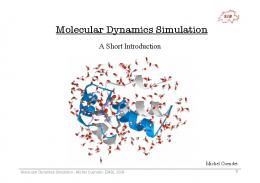
the String Method [5], the latter of which performs simulations on multiple replica systems. MDL is built with the scripting language Python, providing a set of high-level application programming interfaces (APIs) which are domainspecific and enable construction of new propagators, force calculators, and high level sampling protocols which can be tested through simulation protocol scripts. MDL invokes lower-level precompiled C++ libraries from ProtoMol [6] wrapped with SWIG [7] for Python, as shown in Figure 1. ProtoMol is an object-oriented and extensible C++ framework for conducting MD simulations, which uses many object-oriented design patterns [8]. Functionality from ProtoMol which is common to many MD simulations and does not require prototyping in the scripting language is precompiled into machine code to save performance. Development can be done through the Eclipse [9] Interactive Development Environment (IDE) by downloading PyDev [10] plugins, and scripts can be run through the IPython [11] interpreter which offers command shell access, tab-completion and easier debugging. More recently, application of Graphics Processing Units (GPUs) in computationally intensive MD simulations has become an important area of research [12]. Modern GPUs far exceed CPUs in terms of raw computing power. GPU implementation of MD simulation methods can provide a performance gain of one or two orders of magnitude over the best CPU implementations. However, GPUs differ from CPUs in many fundamental ways that impact how GPUs can be programmed, and considerable challenges exist in capturing the parallelism of a GPU while running MD simulations. Given that new MD simulation methods are also being developed on the GPUs, reusability of the GPU implementations is essential. OpenMM [13] falls under this category as an open-source, extensible API for molecular mechanics. OpenMM provides a set of C++ libraries for force calculation, which invoke routines in the CUDA [14] or Brook [15] APIs. These tools are responsible for distributing computation to high-performance GPUs. We interface MDL with OpenMM, allowing users to capture the massive speedup provided by GPUs. To further facilitate testing, MDL includes interfaces to external Python libraries for plotting and data analysis. The MDL framework is available open source at http://mdlab.sourceforge.net. The Molecular Modeling Toolkit (MMTK, [16]) is also built with Python and is well-suited for simulation protocols, providing easy access to system attributes and like MDL incorporates parallelism. For propagating, MMTK provides a Velocity Verlet propagator [17] which can be customized accordingly for general constant energy, constant temperature (using a Nosé thermostat, [18]) or constant pressure (using an Andersen Barostat, [19]) integration. While MMTK is general purpose, MDL is more specific to the actual development of new simulation methods, representing low-level data as Numerical Python (NumPy, [20]) vectors and matrices and enabling easy integration with simulation protocols. Many scientific developers prefer the extensive number crunching libraries available in Matlab particularly with its impressive Interactive Development Environment (IDE). Python provides enough flexibility and ac3

Fig. 1. Architecture of MDL and ProtoMol. Each can be developed independently, using an IDE such as Eclipse. We wrap ProtoMol modules for MDL using SWIG, producing (dark arrow) a set of precompiled shared objects and Python wrappers which invoke (clear arrow) functionality within these shared objects. We also wrap calls to the OpenMM libraries which in turn invoke routines from the CUDA or Brook APIs, and distribute computation across high-performance GPUs. Calls to the MDL API will either invoke pure Python or the Python wrappers, and simulation observables can then be ported to external tools for plotting, visualization, etc.

cess to facilities not meant for number crunching, and better syntactic balance between mathematical constructs and domain specificity. Moreover since the Python interpreter executes in the C runtime environment and a Python/C API is available, the interface between Python and C is cleaner. This provides opportunities to optimize simulations by including expensive algorithms as precompiled libraries. In addition, there are many external tools built with Python and as a result compatible with MDL. We use some of these tools to provide similar number crunching and plotting abilities that could be achieved with Matlab, and others for optimizations such as parallelism. Python and MDL are also more readily available, as they can be downloaded open source for Linux, Macintosh and Windows platforms. We published a preliminary version of MDL in [21]. Here we present a new package with improved organization, more capabilities including an interface to a Java Graphical User Interface (GUI), better exception handling, more flexibility, and better ability to perform computationally demanding sampling through OpenMM. Moreover, we present a wider range of examples, an imple4

mentation of the improved On-The-Fly String Method [5], and performance comparisons with standalone ProtoMol.

2

MDL Simulation Protocols

The best way to test accuracy and stability of a new simulation method is to set up an MDL simulation protocol, which through the MDL API sets up a physical system, forces to evaluate, observables to examine, and the propagator. The MDL API is also invokable within the simulation method itself and consists of a set of core classes which hold different types of information for MD simulations: (1) Physical: The physical system, including all coordinate and structural information (position and velocity vectors, mass matrices, temperature, etc.) (2) ForceField: The set of forces (e.g., dihedral and electrostatics) and algorithms (e.g., cutoff or Particle Mesh Ewald) to evaluate them. (3) Forces: Holds data for the atomic force vector and system energies. (4) IO: Functionality for populating a system through file input, and various forms of data analysis output including plots, files and the screen. (5) Propagator: Functionality to propagate the system, including dynamical integrators and Monte Carlo methods.

2.1 Physical System The first step for most simulation protocols will be to construct an instance of the MDL class Physical, representing the physical system. Once this instance has been constructed, its member attributes can be set directly through the dot operator, or with the help of the MDL class IO. In Listing 1 we show the construction of an 1101-atom solvated Bovine Pancreatic Tripsin Inhibitor [22] system: Listing 1. Setting up a physical system. 1 2 3 4 5 6 7

phys = Physical ( ) io = IO ( ) io . r e a d P D B P o s( phys , " data / b p t i _ w a t e r _ 1 1 0 1 / bpti . pdb " ) io . readPSF ( phys , " data / b p t i _ w a t e r _ 1 1 0 1 / bpti . psf " ) io . readPAR ( phys , " data / b p t i _ w a t e r _ 1 1 0 1 / bpti . par " ) phys . bc = " Periodic " phys . t e m p e r a t u r e = 300

5

Although in this particular case we choose to call the object phys, any valid Python variable name can be used. We use file input to populate phys by invoking member functions of MDL class IO. MDL supports data formats popular in the MD community, including coordinate files from the Protein Data Bank (PDB, [23]), CHARMM 27 [24,25] Protein Structure Files (PSFs) and Parameter (PAR) files, Gromacs [26] topology files and AMBER [27] force fields. Several example physical systems are included with MDL. Other attributes of phys can then be manually set, such as boundary conditions and temperature in Kelvin.

2.2 Force Computation

MD forces can be classified as bonded (between nearby covalently bonded atoms) and nonbonded (between atoms which are not covalently bonded). MDL directly supports CHARMM [24,25] and AMBER [27] force fields, which consist of four types of bonded forces contributing from deviations of twoatom bonds, three-atom angles and four-atom dihedrals and impropers from equilibrium values; and two types of nonbonded forces due to the LennardJones (Pauli Exclusion and van der Waals terms) and electrostatic potentials shown in Eq. (2), where r represents the pairwise distance between two atoms. VLJ = 12

A B −6 6 , 12 r r

VCoulomb =

kq1 q2 . r2

(2)

In Listing 2 we construct instances of the MDL Forces and ForceField classes, instructing the latter to evaluate all six forces from the CHARMM force field and populate the former. Listing 2. Setting up MDL forces. 1 2 3 4 5 6 7 8 9

forces = Forces ( ) ff = forces . m a k e F o r c e F i e l d ( phys , " charmm " ) ff . params [ " L e n n a r d J o n e s" ] = { ' a l g o r i t h m ' : ' Cutoff ' , ' s w i t c h i n g ' : ' C2 ' , ' switchon ' : 8 .0 , ' cutoff ' : 12 . 0 } ff . params [ " Coulomb " ] = { ' a l g o r i t h m ' : ' Cutoff ' , ' s w i t c h i n g ' : ' C1 ' , ' cutoff ' : 12 . 0 }

Nonbonded pairwise forces are usually computed using a cutoff. By using a cutoff of 12 ˚ A for electrostatic calculations, some of this computation can be saved by assuming zero force if two atoms have a pairwise distance greater 6

than this cutoff. In addition, we use a first-order continuous switching function and apply it to the potential curve for stability at the cutoff value. For Lennard-Jones we use a second-order continuous switching function and begin its application at a distance of 8 ˚ A, up to the cutoff of 12 ˚ A. Since we are using periodic boundary conditions, a cubic box is superimposed and the minimal image convention is used to determine pairwise distance between atoms. As an alternative, one could incorporate Particle Mesh Ewald (PME, [28]) approximation to the electrostatic force computation for better accuracy, as shown in Listing 3. MDL also includes implicit solvent algorithms such as SCPISM [29] and Generalized Born [30]. Listing 3. Incorporating the Particle Mesh Ewald approximation. 1 ff . params [ ' Coulomb ' ] = { ' a l g o r i t h m ' : ' PME ' , 2 ' s w i t c h i n g ' : ' Cutoff ' , 3 ' gridsize ' : 15 , 4 ' cutoff ' : 12 }

2.3 Output For observable output, the MDL IO class provides functionality for both instantaneous and trajectory output, in multiple formats (files, plots, and the screen). For example, Listing 4 shows the assignment of io.screen to a frequency of 2. Listing 4. Initializing screen output. 1 io . screen = 2

This prints step number, femtosecond time, total energy, and temperature to the screen every two steps of propagation, formatted according to the following sample: Step: 0, Time: 0.000 [fs], TE: 198.0526 [kcal/mol], T: 308.2064 [K] Step: 2, Time: 40.000 [fs], TE: 198.0234 [kcal/mol], T: 302.3148 [K] Step: 4, Time: 80.000 [fs], TE: 198.0834 [kcal/mol], T: 284.0183 [K] ... We can also plot observables by accessing the plots data member dictionary of the IO class, which maps Python strings to integer frequencies. Plotting is performed through external libraries. MDL provides interfaces to both Gnuplot-py [31] and Matplotlib [32]. Gnuplot-py interacts with Gnuplot [33] which comes standard on many versions of *nix, and Matplotlib provides an environment similar to Matlab [34]. Gnuplot-py is the default, but we can 7

switch to Matplotlib by setting the useMPL boolean data member of IO to true. For example, the code in Listing 5 plots pressure every five steps and total energy every two: Listing 5. Initalizing an MDL plot. 1 io . useMPL = True 2 io . plots = { ' pressure ' :5 , ' t o t a l e n e r g y ' : 2 }

For trajectory file output, MDL can generate Matlab-compatible data in tabular format, with the first column containing step number and subsequent columns containing observable values. MDL can also generate trajectory force, position or velocity vectors in XYZ or binary DCD format. Trajectory file output is performed by accessing the files data member of class IO, which maps strings to Python pairs of filenames and frequencies. In addition, the MDL IO class contains member functions for instantaneous file output in PDB or XYZ format, as shown in Listing 6. Listing 6. Initializing file I/O. 1 io . files = { ' energies ' : ( ' energies . out ' , 2 ) 2 ' d c d t r a j p o s ' : ( ' p o s i t i o n s. out . dcd ' , 5 ) , 3 ' x y z t r a j v e l ' : ( ' v e l o c i t i e s. out . xyz ' ,1 ) } 4 io . w r i t e P D B P o s( phys , " p o s i t i o n s. pdb " ) 5 io . w r i t e X Y Z V e l( phys , " v e l o c i t i e s. xyz " )

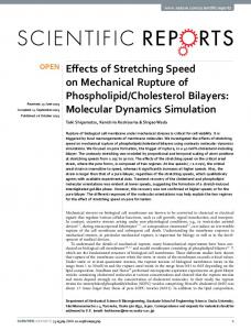
Finally, the system can be viewed interactively through the Java Molecular Viewer (JMV) GUI of ProtoMol, available open source. Instructions for download are available on the MDL website. By setting the gui data member of class IO to the appropriate frequency as shown in Listing 7, structural and positional information is sent to the GUI through port 52753 on your local host. Figure 2 shows an MDL simulation viewed through the JMV. Listing 7. Initializing the interactive GUI. 1 io . gui = 3

2.4 Propagation An MDL propagator can be initialized as shown in Listing 8.

8

Fig. 2. Screenshot of the Java Molecular Viewer, running an MDL simulation of alanine dipeptide in vacuum. Listing 8. Initializing an MDL propagator. 1 prop = P r o p a g a t o r( phys , forces , io )

Once constructed, the passed Physical object is updated for a specific number of steps upon a call to the Propagator member function propagate. For example, Listing 9 runs 1 ps of Leapfrog. Listing 9. Execution of 1 ps of Leapfrog. 1 prop . p r o p a g a t e( scheme = ' Leapfrog ' , steps = 2000 , 2 dt = 0 .5 , f o r c e f i e l d= ff )

One can also use Normal Mode Langevin (NML, [35]) for propagation. NML allows one to partition the degrees of freedom of the system into a set of fast and slow frequency components. One can propagate along the set of slow frequency components while performing over-damped dynamics along the fast frequency components. Note that the timestep of integration for a system is bounded by the highest frequency component. Therefore, NML allows one to take a larger timestep for propagation. NML is implemented as a multiple timestepping (MTS) integrator. The outermost propagator NormalModeDiagonalize computes the mass-reweighted Hessian of the system and diagonalizes the Hessian matrix to obtain a set of normal mode eigenvectors and correspond9

ing eigenvalues. The eigenvalues determine the frequency associated with each eigenvector. This process is performed at a diagonalization frequency in steps. Diagonalization can be performed using an O(N log N) coarse-grained procedure. This is indicated by the parameter fullDiag=False. Setting autoParameters=True estimates the best parameters for the coarse grained diagonalization [36]. NormalModeLangevin runs Langevin dynamics along the set of slow frequency modes while the bottom integrator NormalModeMinimizer finds the most probable conformation of the system along fast modes by minimizing potential energy. The former accepts parameters for standard Langevin dynamics (temperature in Kelvin, damping coefficient in ps−1 , random number seed) plus the number of slow modes, while the latter accepts a target potential energy deviation for minimization using mass-reweighted steepestdescent. This propagation scheme is set up in Listing 10. Listing 10. Normal modes in MDL. 1 prop . p r o p a g a t e( scheme = [ ' N o r m a l M o d e D i a g o n a l i z e ' , 2 ' NormalModeLangevin', 3 ' NormalModeMinimizer '] , 4 steps = 20 , c y c l e l e n g t h= [1 , 1 ] , dt = 4 .0 , 5 f o r c e f i e l d= [ ff , ff2 , ff3 ] , 6 params = { ' N o r m a l M o d e D i a g o n a l i z e ' : 7 # Rediagonalization frequency 8 { ' reDiag ' : 100 , 9 ' fullDiag ' : False , 10 ' a u t o P a r a m e t e r s ' : True } , 11 ' NormalModeLangevin': 12 # Number of slow modes 13 { ' n u m b e r m o d e s ' : 22 , 14 ' gamma ' : 80 , # Langevin 15 ' seed ' : 1234 , 16 ' t e m p e r a t u r e ' : 300 } , 17 ' NormalModeMinimizer ': 18 # Target PE diff , kcal / mol 19 { ' minimlim ' : 0 . 2 } )

To use the processing power of GPUs, MDL includes the OpenMM propagator which runs Langevin dynamics and is set up with default parameters as shown in Listing 11. Listing 11. Execution of 1 ps of Langevin dynamics on GPUs. 1 prop . p r o p a g a t e( scheme = ' OpenMM ' , steps = 2000 , 2 dt = 0 .5 , f o r c e f i e l d= ff )

10

This default version of OpenMM evaluates all six AMBER [27] forces (bond, angle, dihedral, improper, LennardJones and electrostatic), although a subset can be evaluated by changing parameters. The OpenMM propagator evaluates these forces by invoking routines included with the OpenMM libraries. These routines then invoke routines in the CUDA or Brook APIs which handle distributing the computation to GPUs, assuming the installation of a compatible graphics card. In addition, electrostatic forces can be approximated using the Generalized Born (GB) [30] implicit solvent model by setting the gbsa member of MDL class ForceField to True, as shown in Listing 12. If GB is to be used, Gromacs topology and AMBER force fields must be used to set up the physical system, as essential GB parameters are included in these files. In Section 3.5 when we evaluate performance, we illustrate the potentially large savings in execution time for computationally demanding sampling of large-scale systems using OpenMM on GPUs vs. CPUs, using an NVIDIA [37] graphics card. Listing 12. Specification of Generalized Born as the algorithm for evaluating electrostatic forces. 1 ff . gbsa = True

Several propagators are predefined and already included in the MDL package, and these along with their uniquely identifying Python strings and parameter values plus defaults are included on the MDL webpage. We also include in the Appendix a list of the propagators available in MDL along with their appropriate ensembles; and in this same table include different force calculators that are available for electrostatics and some propagator modifiers. In addition to the available propagators, users can define new propagators as Python classes or functions and assign them names, parameter values and defaults. We now illustrate this.

3

Prototyping simulation methods

3.1 Propagators MDL provides flexibility with constructing new propagators, allowing implementation as a Python class for users more familiar with object-oriented programming, or a Python function for those who prefer a procedural style. Either construct should be defined in its own Python module, which must include bindings between a variable name and a uniquely identifying Python string, and between a variable parameters to a possibly empty Python tuple of parameter names and default values. For example, if we were to create a new 11

BBK [38] propagator which runs Langevin dynamics, our bindings might look something like Listing 13. Listing 13. Registering a new BBK propagator. 1 name = " BBK " 2 p a r a m e t e r s= ( " temp " , 300 , " gamma " , 0 .5 , " seed " , 1234 )

The same Python string bound to name is passed in the call to propagate() when the new scheme is used. 3.2 Classes MDL propagator classes inherit from one of two interfaces: STS for single timestepping and MTS for multiple. Returning to the BBK example, we can inherit from STS and define an init() method which calculates forces, as shown in Listing 14. Listing 14. init() method of the new BBK propagator. 1 class BBK ( STS ) : 2 def init ( phys , forces , prop ) : 3 prop . c a l c u l a t e F o r c e s ( forces )

The first half of the BBK propagator can be represented by Eq. (3), where F, V and X are respectively the atomic force, velocity and position vectors, M the atomic mass matrix and FR a random force. Thus the method incorporates a random force and provides some initial velocity damping, before performing a half-timestep velocity update and full-timestep update of positions. V n+1/2 = V n (1.0 −

∆t γ) 2

+

∆t M −1 (F n 2

X n+1 = X n + V n+1/2 ∆t.

+ FR

q

2kT γ ) ∆t

(3)

When we implement these equations in the run() method as shown in Listing 15, we gain access to the atomic data as attributes of the Physical object formal parameter which are represented as Numpy arrays and matrices and thus mathematical operations can be performed on those structures as a whole. Any parameters that were defined become bound as member variables of class BBK and are accessible as attributes of self:

12

Listing 15. Implementation of Eq. (3) in MDL. 1 2 3 4 5 6 7 8 9

def run ( self , phys , forces , prop ) : f o r c e c o n s t a n t = 2 * C o n s t a n t s. b o l t z m a n n( ) * self . temp * self . gamma / self . dt forces . force + = forces . r a n d o m F o r c e( self . seed ) * sqrt ( f o r c e c o n s t a n t) phys . v e l o c i t i e s * = 1 . 0 - 0 . 5 * self . dt * self . gamma phys . v e l o c i t i e s + = 0 . 5 * self . dt * phys . i n v m a s s e s * forces . force phys . p o s i t i o n s + = phys . v e l o c i t i e s* self . dt

Then after a recalculation of forces, the second half of BBK incorporates another random force term and performs a final half-timestep update on velocities, as shown in Eq. (4).

V n+1 = (V n+1/2 +

∆t M −1 (F n+1 2

+ FR

q

2kT γ ))(1/(1.0 ∆t

+

∆t γ)). 2

(4)

Continuing in the implementation of run(), we recalculate forces in the same way as init(), once again by adding the random force to the atomic force vector, and using these resulting force values to update the atomic velocity vector. We show this in Listing 16. Listing 16. Implementation of Eq. (4) in MDL. 1 2 3 4 5 6

prop . c a l c u l a t e F o r c e s ( forces ) forces . force + = forces . r a n d o m F o r c e( self . seed ) * sqrt ( f o r c e c o n s t a n t) phys . v e l o c i t i e s + = 0 . 5 * self . dt * phys . i n v m a s s e s * forces . force phys . v e l o c i t i e s * = ( 1 / ( 1 . 0 + 0 . 5 * self . dt * self . gamma ) )

One could use an analogous approach to constructing propagators which require a second set of positions and velocities, such as Nosé-Hoover [18] or Nosé-Poincaré [39] which impose thermostats. Additional sets of physical coordinates can be implemented as members of the appropriate propagator class, which can then evolve both the MDL Physical coordinates and its data member coordinates. Python class implementations of Nosé-Poincaré and Recursive Multiple Thermostatting (RMT, [40]) which applies the Nosé thermostat multiple times are available on the MDL webpage. 13

3.2.1 Modifiers In some cases, a new propagator may consist of the exact same implementation as an existing propagator object, with slight modifications in specific locations of the propagation. To avoid defining a new class, MDL provides modifier functions which can be classified according to the point of invocation and invoked transparently at the correct times. Modifier classifications include: PreInit, PostInit, PreForce, PostForce, PreRun and PostRun. Thus the control flow of an MDL propagator object proceeds as shown in Figure 3.

Fig. 3. Diagram illustrating the control flow of MDL propagator objects, including the points of modifier invocations.

As an example, if we wanted to modify the Leapfrog propagator to model NVT dynamics through an artificial scaling of velocities to keep average kinetic energy KE = 23 NkT constant, we could implement as a PostRun modifier a function which scales velocities, then simply define a new propagator VelocityScale as a subclass of Leapfrog, with one extra parameter and the VelocityScale modifier included. Modifiers are specified by binding a Python variable modifiers to a set of tuples of modifier names and types, as shown in Listing 17. Listing 17. Implementation of a modifier for NVT dynamics. 1 def s c a l e V e l o c i t i e s ( phys , forces , prop , obj ) : 2 phys . v e l o c i t i e s * = numpy . sqrt ( obj . T0 / phys . t e m p e r a t u r e( ) ) 4 class V e l o c i t y S c a l e( Leapfrog ) : pass 6 name = " V e l o c i t y S c a l e" 7 p a r a m e t e r s= ( ' T0 ' , 300 ) 8 m o d i f i e r s = [ ( " s c a l e V e l o c i t i e s " , " PostRun " ) ]

14

3.3 Functions

MDL propagators can also be represented as Python functions. A propagator function may also accept a function handle for the next propagator in the chain and its arguments, if the propagator is MTS. Thus the structure of the function itself is very similar to the analogous propagator object. The run() method would be equivalently implemented in a counter-controlled Python for loop with the iteration count equal to the number of steps. The init() method functionality would be placed before this loop. With this in mind, the BBK propagator would look like Listing 18 as a Python function. Listing 18. Implementation of BBK as a function. 1 def bbk ( phys , forces , io , steps , timestep , fg , 2 temp , gamma , seed ) : 3 fg . c a l c u l a t e F o r c e s ( phys , forces ) # init 5 6 7 8 9 10 11 12 13 14 15 16

for step in range (0 , steps ) : # run fc = 2 * C o n s t a n t s. b o l t z m a n n( ) * temp * gamma / timestep forces . force + = forces . r a n d o m F o r c e( phys , seed ) * sqrt ( fc ) phys . v e l o c i t i e s * = ( 1 . 0 - 0 . 5 * timestep * gamma ) phys . v e l o c i t i e s + = forces . force * 0 . 5 * timestep * phys . i n v m a s s e s phys . p o s i t i o n s + = phys . v e l o c i t i e s* timestep fg . c a l c u l a t e F o r c e s ( phys , forces ) forces . force + = forces . r a n d o m F o r c e( phys , seed ) * sqrt ( fc ) phys . v e l o c i t i e s + = forces . force * 0 . 5 * timestep * phys . i n v m a s s e s phys . v e l o c i t i e s * = ( 1 . 0 / ( 1 . 0 + 0 . 5 * timestep * gamma ) )

3.4 Force Calculators

In addition to propagators, new force calculators can be prototyped as Python classes. A force calculator must minimally define a Python constructor and an evaluate() method which accepts no parameters and returns nothing but accesses and modifies these objects, particularly the atomic force vector and energies structures. For example, we could define the harmonic dihedral restraint shown in Eq. (5), where φi (~x) represents the value of a selected dihedral i and φ0 represents a target value in radians around which φi (~x) should harmonically oscillate. The constant k controls the restraint strength. V (~x) = k(φi (~x) − φ0 )2 .

(5) 15

We can define a new class HDForce to implement this potential term and update the atomic force vector. We must first define its constructor as shown in Listing 19, which initializes member variables. Listing 19. Definition of a class HDForce to represent an MDL force calculator. 1 class HDForce : 2 def __init__ ( self , phys , forces , phi , num , k ) : 3 self . phys = phys , self . forces = forces , 4 self . phi = phi , self . num = num , self . k = k

Then the responsibility of evaluate is to update the energies and force values contained within the now data member object forces. We compute the potential term by calculating the difference between the appropriate dihedral value and its target and applying wraparound if necessary, then accumulate the result into the system dihedral energy. This is shown in Listing 20. Listing 20. Computation of the dihedral energy. 1 def evaluate ( self ) : 2 diff = self . phys . phi ( self . num ) - self . phi 3 if ( diff < - numpy . pi ) : diff + = 2 * numpy . pi 4 elif ( diff > numpy . pi ) : diff - = 2 * numpy . pi 5 self . forces . energies . a d d D i h e d r a l E n e r g y ( self . k * diff * * 2 )

This potential term will only apply forces to the four atoms i, j, k and l which compose the dihedral. We obtain the appropriate indices and pairwise distances as shown in Listing 21. Listing 21. Computation of the pairwise distances of atoms that compose a dihedral. 1 2 3 4 5 6 7 8 9 10

atomI atomJ atomK atomL rij =

= self . phys . dihedral ( self . dihedral - 1 ) . atom1 = self . phys . dihedral ( self . dihedral - 1 ) . atom2 = self . phys . dihedral ( self . dihedral - 1 ) . atom3 = self . phys . dihedral ( self . dihedral - 1 ) . atom4 self . phys . p o s i t i o n s[ atomJ * 3 : atomJ * 3 + 3 ] - self . phys . p o s i t i o n s[ atomI * 3 : atomI * 3 + 3 ] rkj = self . phys . p o s i t i o n s[ atomJ * 3 : atomJ * 3 + 3 ] - self . phys . p o s i t i o n s[ atomK * 3 : atomK * 3 + 3 ] rkl = self . phys . p o s i t i o n s[ atomL * 3 : atomL * 3 + 3 ] - self . phys . p o s i t i o n s[ atomK * 3 : atomK * 3 + 3 ]

-

1 1 1 1

Then to compute the force on each atom, we must apply chain rule to calculate the gradient of the potential. ∇φ, Fi = − δU δφ 16

We first compute the derivative of the potential term with respect to the angle φ, then use the NumPy cross and dot product functions to calculate the force on each atom, and finally accumulate these forces into the atomic force vector using the atom indices, as shown in Listing 22. Listing 22. Computation of the harmonic dihedral force. 1 2 3 4 5 6 7 8 10 11 12 13

dUdPhi = 2 * self . k * diff A = numpy . cross ( rij , rkj ) B = numpy . cross ( rkj , rkl ) fi = A * ( - dUdPhi * norm ( rkj ) / norm2 ( A ) ) ; fl = B * ( dUdPhi * norm ( rkj ) / norm2 ( B ) ) ; fj = fi * ( - 1 + numpy . dot ( rij , rkj ) / norm2 ( rkj ) ) - fl * ( numpy . dot ( rkl , rkj ) / norm2 ( rkj ) ) ; fk = - ( fi + fj + fl ) ; self . forces . force [ atomI * 3 : atomI * 3 + 3 ] self . forces . force [ atomJ * 3 : atomJ * 3 + 3 ] self . forces . force [ atomK * 3 : atomK * 3 + 3 ] self . forces . force [ atomL * 3 : atomL * 3 + 3 ]

+= += += +=

fi fj fk fl

Python forces can be added to ForceField object by first constructing an instance of the class with the appropriate parameter values passed to the constructor, then passing this instance as a parameter to the ForceField member function addPythonForce, as shown in Listing 23. Listing 23. Instantiation of the harmonic dihedral force object, and its inclusion as a force in our simulation protocol. 1 hd = HDForce ( phys , forces , phi = 3 .0 , num =1 , k = 1 ) 2 ff . a d d P y t h o n F o r c e( hd )

3.5 Comparison with ProtoMol

By comparing the wall clock execution time of MDL simulations against their counterparts in ProtoMol, we can obtain an idea of the types of simulation methods which yield minimal to acceptable performance declines, and determine if any result in large performance penalties. However even a large performance penalty does not necessarily imply computational intractability, since short simulations may be required to test a particular simulation method for accuracy and stability. In Table I, we show the wall clock execution time in seconds of two propagators and two force calculators executed with standalone ProtoMol, MDL with 17

precompiled shared object machine code implementation of the simulation method, and a pure Python implementation of the method. All tests were run on a 2.5 GHz Xeon processor using 16 GB of RAM running Gentoo Linux 2.6.2. We use a 1 ps simulation. For the propagator tests and linear time harmonic dihedral restraint we used a moderately sized 1101-atom solvated BPTI simulation with periodic boundary conditions and a direct evaluation of pairwise forces. For the quadratic electrostatic force calculator, we used an unsolvated alanine dipeptide molecule in vacuum and ran Langevin Impulse. Method

ProtoMol

Wrapped

Python

BBK

46.745 ± 0.124

53.869 ± 0.116

59.481 ± 0.149

Impulse/Leapfrog

25.013 ± 0.188

28.971 ± 0.038

29.459 ± 0.145

Harmonic Dihedral

46.044 ± 0.646

53.386 ± 0.126

53.889 ± 0.791

Electrostatics

0.115 ± 0.004

0.147 ± 0.001

16.122 ± 0.080

Table I. Wall Clock execution times for simulation methods run through ProtoMol, MDL using precompiled machine code, and MDL using pure Python for the method.

This illustrates that non-bottleneck algorithms such as propagators and nonpairwise force calculators yield small performance penalties when prototyped in pure Python, since the bulk of the simulation is still implemented within precompiled machine code. When a pairwise electrostatic force is introduced, the penalty becomes quite large. Part of this penalty is due to the fact that ProtoMol incorporates some optimizations for pairwise evaluations such as cell lists which contain nearby atom pairs, and a future extension could be to build hooks such that these optimizations become available in Pythonprototyped pairwise force calculators as well. In Table II, we evaluate performance savings resulting from running the OpenMM propagator on NVIDIA [37] GPUs vs. running on the CPU. For these tests we use three systems; a 544-atom Fip35 WW mutant [41], a 2262-atom calmodulin system (PDB ID 1CLL), and a 7214-atom tyrosine Kinase system (PDB ID 1QCF). Our simulations use a timestep of 0.5 fs and we run for 10000 steps, a total time of 5 ps. We evaluate all bonded and nonbonded forces and measure wall clock execution time in nanoseconds per day. We compare OpenMM running general Langevin dynamics on GPUs using the Generalized Born implicit solvent model for electrostatics and the OpenMM force calculators with the LangevinImpulse propagator on the CPU using the faster SCPISM implicit solvent model for electrostatics and the optimized force calculators included with ProtoMol. Our goal here is to benchmark an MDL simulation on the GPUs against the best performance available with MDL using the CPU. Results show that running the OpenMM propagator on the GPUs yields considerable savings even compared to the highly optimized force calculators of 18

System

Atoms OpenMM GPU (ns/d)

ProtoMol CPU (ns/d)

GPU Speedup

WW

544

109.04

1.72

65.81

Calmodulin 2262

16.09

0.10

159.81

Tyr Kinase

2.08

0.0094

221.28

7214

Table II. Wall clock execution times of three large-scale systems, running the OpenMM libraries for force calculation on GPUs vs. the ProtoMol libraries on the CPU.

ProtoMol on the CPU; ranging from 65 to 221 fold. With this interface to OpenMM available in MDL, users gain flexibility. For system protocols which require subprocesses that involve computationally demanding sampling of large-scale systems, users can run the OpenMM propagator to take advantage of the speedup provided by GPUs. For protocols that are less computationally intensive and propagate smaller systems, which will often be the case when testing simulation methods such as propagators and force calculators, the interface to the ProtoMol libraries is sufficient. Both OpenMM and ProtoMol are continually developed, and interfaces to their routines are also updated in MDL.

4

Example High-Level Sampling Protocol: Parallel On-The Fly String Method

As an example of a high level simulation protocol that uses full molecular dynamics as steps of its execution we present the On-The-Fly String Method [5], which is an iterative approach to finding the Minimum Free Energy Path (MFEP) between a pair of metastable states of a biomolecule. The String Method operates in a collective space with dimensions in general much smaller than 3N but which can be used to describe a reaction path between the two conformations. The string consists of a set of discrete points on an arbitrary path connecting two states. The String Method updates each point with MD simulation until the string converges to the MFEP. Since the points are evolved independently, the method is parallelizable. We use the On-The-Fly String Method as an example which illustrates the ability of MDL to construct simulation methods modularly, using subprocesses which are themselves simulation methods. This includes the use of our VelocityScale propagator that we constructed in Section 3.2 to evolve the trajectories, and implementing a restraint using our HDForce constructed in Section 3.4. Our implementation incorporates an external tool built with Python for parallelism. 19

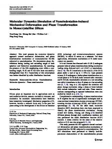
4.1 Implementation We implemented the On-The-Fly String Method in parallel using MDL, executed through an external Python interpreter PyMPI [42] which interfaces to the Message Passing Interface (MPI, [43]). After importing the mpi module, PyMPI recognizes attributes size as the number of processors, rank as the unique identifier of the current processor, and data communication using bcast and allgather. In our parallel implementation, each processor is assigned a set of string points. Dynamics is thus executed on individual processors, and the string is gathered and reparameterized on the master node. We test our implementation of the String Method using alanine dipeptide molecule in vacuum and use the φ − ψ backbone dihedral angle values as collective variables. Figure 4 shows our initial string labeled accordingly, with the two endpoints resting near metastable states defined by the C7-equatorial and C7-axial conformations and the intermediate points equidistant from each other. We obtained the contour levels of the free energy map by dividing collective space into 900 boxes of equal dimension and sampling using constant temperature dynamics and harmonic restraints at the center points of each box, then computing free energy values at different points using the Weighted Histogram Analysis Method (WHAM, [44]). We initialize the endpoints of the string near the two metastable states in Listing 24, at backbone dihedral radian values (-1.87, 2.44) and (1.27, -1.22) on the master node and then scatter the points to all slaves, giving z p a single point on the string z. In this case, 11 and 18 represent the indices of the backbone dihedrals which we reference.

20

Fig. 4. Our initial string, and results of our simulation after 50 ps of alanine dipeptide simulation. Both have been superimposed on the free energy contour plot in collective space. Listing 24. Initialization of our string. 1 2 3 4 5 6 7 8 9 10 11 12 13 14 15 16 17 18

PHI = 11 , PSI = 18 if ( mpi . rank = = 0 ) : z = [ ] # EMPTY STRING # INITIAL AND FINAL POINTS phiI = - 1 . 87 , psiI = 2 . 44 phiF = 1 . 27 , psiF = - 1 . 22 # INTERIORS z . append ( [ phiI , psiI ] ) newphi = phiI , newpsi = psiI for ii in range (1 , n u m p o i n t s- 1 ) : newphi + = ( phiF - phiI ) / ( n u m p o i n t s- 1 ) newpsi + = ( psiF - psiI ) / ( n u m p o i n t s- 1 ) z . append ( [ newphi , newpsi ] ) z . append ( [ phiF , psiF ] ) else : z = [] # SCATTER POINTS TO ALL SLAVES z_p = mpi . scatter ( z )

21

To propagate the string z, Maragliano et al. moved every point in the direction of the mean force acting at that point in collective space, which will involve a change of variables from Cartesian space. They propagate two independent replicas x and y using MD with harmonic restraints on the backbone dihedrals, which are the same as our prototyped HDForce. At each point p, the string is updated according to Eq. (6), where κ is the harmonic dihedral restraint control parameter, γ controls the rate of string propagation, and Mij is a scalar tensor which is defined by Eq. (7), where n is the number of atoms in the system. This performs the projection of the gradient of the potential energy U(x) into a V (φ(x), ψ(x)) in collective space. zφp − = zψp − =

κ∆t [Mφφ (xp )(zφp γ κ∆t [Mψφ (xp )(zφp γ

Mαβ (x) =

− φ(y p)) + Mφψ (xp )(zψp − ψ(y p ))] − φ(y p )) + Mψψ (xp )(zψp − ψ(y p ))],

n X

1 δα(x) δβ(x) δxk k=1 mk δxk

(6)

(7)

We create a Python function to compute M which involves similar computation of dihedral derivatives as our HDForce prototype. Then on each node we update the string points accordingly, as shown in Listing 25. Listing 25. Update of the string points. 1 zp0 = z_p [ 0 ] 2 z_p [ 0 ] - = ( kappa * dt / gamma ) * ( M (x , PHI , PHI ) 3 * ( z_p [ 0 ] - y . angle ( PHI ) ) 4 + M (x , PHI , PSI ) 5 * ( z_p [ 1 ] - y . angle ( PSI ) ) ) 6 z_p [ 1 ] - = ( kappa * dt / gamma ) * ( M (x , PSI , PHI ) 7 * ( zp0 - y . angle ( PHI ) ) 8 + M (x , PSI , PSI ) 9 * ( z_p [ 1 ] - y . angle ( PSI ) ) )

We then set up the MD replica on each node, as illustrated earlier using CHARMM force fields, vacuum boundary conditions and direct computation of pairwise forces. We then add our Python-prototyped harmonic dihedral restraint twice, once for φ and once for ψ, and set up two propagators px and py to propagate two MDL Physical objects x and y which have been initialized with the same data. Finally, we propagate using our NVT VelocityScale propagator (constructed earlier) at 300 K, as shown in Listing 26.

22

Listing 26. Execution of dynamics on each MD replica. 1 2 3 4 5 6

ff . a d d P y t h o n F o r c e( HDForce ( angle = z_p [ 0 ] , num = PHI , k = kappa ) ) ff . a d d P y t h o n F o r c e( HDForce ( angle = z_p [ 1 ] , num = PSI , k = kappa ) ) px . p r o p a g a t e( scheme = " V e l o c i t y S c a l e" , steps =1 , dt = dt , f o r c e f i e l d= ff , params = { ' T0 ' : 300 } ) py . p r o p a g a t e( scheme = " V e l o c i t y S c a l e" , steps =1 , dt = dt , f o r c e f i e l d= ff , params = { ' T0 ' : 300 } )

The final step is to reparameterize the string such that all points are an equal arc length apart, to ensure adequate sampling of the entire string. We implement the same algorithm of Maragliano et al. within a function reparam, and execute this only on the master node before once again scattering the new points back to the slaves. This process is shown in Listing 27. Listing 27. Reparameterization of the string, and redistribution of the points across processors. 1 z = mpi . gather ( z_p ) 2 if ( mpi . rank = = 0 ) : reparam ( z ) 3 z_p = mpi . scatter ( z )

We plot the Root-Mean-Square-Deviation (RMSD) of the current string from the initial string, shown in Figure 5(a). This illustrates convergence of the string after about 15 ps of dynamics. We run the simulation for a total of 50 ps and show the results superimposed on a free energy contour in Figure 4 labelled convergence, where the area in green represents the area sampled by the string after convergence and the blue string its average value throughout that time.

Fig. 5. (a) RMSD between our current string value and initial string at each step. (b) Execution times of our implementation of the On-The-Fly String Method in parallel, running a total of 2 ps of dynamics on the solvated alanine dipeptide molecule. (c) Scalability plot of processor count vs. total execution time over all processors.

23

4.2 Parallel Scalability We now test the scalability of our parallel implementation of the On-The-Fly String Method using a 2 ps simulation of solvated alanine dipeptide. Although this was well short of string convergence, this was not necessary to obtain an idea of how well our algorithm scales with processor count. We use a string with 8 replicas which is an adequate amount for sampling collective space between the two metastable states for solvated alanine dipeptide [5]. For simplicity, we allow each node to propagate the same number of string points. Thus we use processor counts of 1, 2, 4 and 8. We show results in Figure 5(b). Results indicate that for a system where dynamics is the bottleneck, our implementation achieves almost complete scalability, as shown by Figure 5(c) which illustrates a near straight-line graph for total execution time (over all processors) vs. processor count. Although this particular example did not require a large number of processors, it does illustrate the potential of a Python based prototyping library to take full advantage of the many libraries of Python. Indeed, other parallel libraries for Python can be used.

5

Conclusions and Future Work

We have presented MDLab as a tool for prototyping, testing and debugging MD simulation methods and tested it through the development of propagators, force calculators, and the more complex On-The-Fly String Method which combines many of our prototyped simulation methods. Building the framework with Python enabled fast construction of new methods, and external tools allowed different types of data analysis and parallelism. MDL thus provides a platform of choice for a simulation method developer to quickly prototype their own method (fast/approximate algorithm for propagation, force calculation, etc.) and test it using biologically relevant systems. Sampling of smaller molecules can be performed through propagation schemes defined by the user, and for more computationally demanding sampling, particularly of large systems, we provide access to OpenMM libraries which capitalize upon the processing power of GPUs. MDL currently uses PyMPI for parallel execution. However, it does not take advantage of parallelism in the back end. This could be addressed in future versions. Although MDL can be run through a PyMPI interpreter to incorporate parallelism, spatial and atom decomposition have been incorporated in the libraries of the ProtoMol back end and is currently inaccessible from PyMPI since the executable passed to MPICH is PyMPI itself. Although we could not simply replace the SWIG-wrapped calls to pairwise force calculations due to the resulting performance decline of serial runs, we could reimplement 24

these algorithms in Python and interface to PyMPI modules, and allow users with access to computing clusters to choose between implementations. This will make parallelism more powerful for the bottleneck calculations. Another challenge involves force calculator prototyping. Prototyping nonbonded force calculation algorithms is limited by the lack of exposure of data structures from the ProtoMol and OpenMM back ends, such as cell and neighbor lists. Exposing these to the MDL API would significantly add expressive power to design new algorithms. Similar gains would be realized by exposing methods for computing analytical and numerical second derivatives.

Acknowledgments This material is based upon work partially supported by grants DBI-0450067, CCF-0135195, and CCF-0622940 to JAI from the National Science Foundation. Thanks to Vijay S. Pande and personnel at Stanford’s NIH Center for Biomedical Computation SIMBIOS for help with interfacing to OpenMM.

25

6

Appendix

Method

Type

BBK [38]

Propagator (NVT)

Langevin Impulse [45]

Propagator (NVT)

NML [35]

Propagator (NVT)

Nosé-Hoover [18]

Propagator (NVT)

Nosé-Poincaré [39]

Propagator (NVT)

OpenMM [13]

Propagator (NVT)

RMT [40]

Propagator (NVT)

Takahashi-Imada [46]

Propagator (NVT)

Leapfrog (Velocity Verlet) [1]

Propagator (NVE)

Position Verlet [17]

Propagator (NVE)

NPT Verlet [17]

Propagator (NPT)

Simple Full

Electrostatic Force Calculator

Cutoff


SCPISM [29]


Generalized Born [30]


Ewald [47]


Particle Mesh Ewald [28]


MultiGrid Summation [48]


Shadow [49]

Modifier

Shake [50]

Modifier

Rattle [51]

Modifier

Table III. Table of the features available in MDL; including propagators/ensembles, force calculators and modifiers. Other simulation methods of these types can be prototyped in Python.

26

References [1] R. W. Hockney, J. W. Eastwood, Computer Simulation Using Particles, McGraw-Hill, New York, 1981. [2] Q. Ma, J. A. Izaguirre, R. D. Skeel, Verlet-I/r-RESPA/Impulse is limited by nonlinear instability, SIAM J. Sci. Comput. 24 (6) (2003) 1951–1973. [3] T. Schlick, Molecular Modeling and Simulation - An Interdisciplinary Guide, Springer-Verlag, New York, NY, 2002. [4] L. Kalé, R. Skeel, M. Bhandarkar, R. Brunner, A. Gursoy, N. Krawetz, J. Phillips, A. Shinozaki, K. Varadarajan, K. Schulten, NAMD2: Greater scalability for parallel molecular dynamics, J. Comput. Phys. 151 (1999) 283– 312. [5] L. Maragliano, E. van den Eijnden, On-the-fly string method for minimum free energy paths calculation, Chem. Phys. Lett. 446 (1–3) (2007) 82–90. [6] T. Matthey, T. Cickovski, S. S. Hampton, A. Ko, Q. Ma, M. Nyerges, T. Raeder, T. Slabach, J. A. Izaguirre, ProtoMol: An object-oriented framework for prototyping novel algorithms for molecular dynamics, ACM Trans. Math. Softw. 30 (3) (2004) 237–265. [7] D. M. Beazley, SWIG: An easy to use tool for integrating scripting languages with C and C++, in: Proceeding of The Forth Annual Tcl/Tk Workshop ’96, USENIX Association, 1996, pp. 129–139. [8] E. Gamma, R. Helm, R. Johnson, J. Vlissides, Design Patterns: Elements of Reusable Object-Oriented Software., Addison-Wesley, Reading, Massachusetts, 1995. [9] Eclipse, Eclipse interactive development environment, http://www.eclipse. org/ (2007). [10] PyDev, PyDev webpage, http://pydev.sourceforge.net/ (2007). [11] IPython, IPython webpage, http://ipython.scipy.org/moin/ (2007). [12] J. E. Stone, J. C. Phillips, P. L. Freddolino, D. J. Hardy, L. G. Trabuco, K. Schulten, Accelerating molecular modeling applications with graphics processors, J. Comp. Chem. 28 (2007) 2618–2640. [13] M. S. Friedrichs, P. Eastman, V. Vaidyanathan, M. Houston, S. LeGrand, A. L. Beberg, D. L. Ensign, C. M. Bruns, V. S. Pande, Accelerating molecular dynamic simulation on graphics processing units, J. Comp. Chem. 30 (6) (2009) 864–872. [14] CUDA, CUDA Zone: The resource for CUDA developers, http://www.nvidia. com/objects/cuda_home.html (2009). [15] Stanford University, BrookGPU, http://www-graphics.stanford.edu/projects/brookgpu/ (2004).

27

[16] K. Hinsen, The molecular modeling toolkit: A new approach to molecular simulations, J. Comp. Chem. 21 (2000) 79–85. [17] W. Swope, H. Andersen, P. Berens, K. Wilson, A computer simulation method for the calculation of equilibrium constants for the formation of physical clusters of molecules: application to small water clusters, J. Chem. Phys. 76 (1982) 637– 649. [18] S. Nosé, A unified formulation of the constant temperature molecular dynamics methods, J. Chem. Phys. 81 (1) (1984) 511–519. [19] H. C. Andersen, Molecular dynamics simulations at constant pressure and/or temperature, J. Chem. Phys. 72 (1980) 2384–2393. [20] NumPy, Numerical Python Libraries, http://numeric.scipy.org (2005). [21] T. Cickovski, C. Sweet, J. A. Izaguirre, MDL, a domain-specific language for molecular dynamics, in: Proc. of the 40th Annual Simulation Symposium ANSS 07, 2007, pp. 256–266. [22] J. Deisenhofer, W. Steigemann, Crystallographic refinement of the structure of bovine pancreatic trypsin inhibitor at 1.5 ˚ A resolution, Acta Cryst. B 31 (1975) 238. [23] F. C. Bernstein, T. F. Koetzle, G. J. Williams, E. F. Meyer, M. D. Brice, J. R. Rogers, O. Kennard, T. Shimanouchi, M. Tasumi, The Protein Data Bank: A computer-based archival file for macromolecular structures, J. Mol. Biol. 112 (1977) 535–542. [24] A. D. MacKerell Jr., D. Bashford, M. Bellott, R. L. Dunbrack Jr., J. Evanseck, M. J. Field, S. Fischer, J. Gao, H. Guo, S. Ha, D. Joseph, L. Kuchnir, K. Kuczera, F. T. K. Lau, C. Mattos, S. Michnick, T. Ngo, D. T. Nguyen, B. Prodhom, B. Roux, M. Schlenkrich, J. Smith, R. Stote, J. Straub, M. Watanabe, J. Wiorkiewicz-Kuczera, D. Yin, M. Karplus, Self-consistent parameterization of biomolecules for molecular modeling and condensed phase simulations, FASEB J. A143 (1992) 6. [25] B. R. Brooks, R. E. Bruccoleri, B. D. Olafson, D. J. States, S. Swaminathan, M. Karplus, CHARMM: A program for macromolecular energy, minimization, and dynamics calculations, J. Comp. Chem. 4 (2) (1983) 187–217. [26] H. J. C. Berendsen, D. van der Spoel, R. van Drunen, GROMACS: A messagepassing parallel molecular dynamics implementation, Comput. Phys. Commun. 91 (1995) 43–56. [27] P. K. Weiner, P. A. Kollman, AMBER: Assisted model building with energy refinement. A general program for modeling molecules and their interactions, J. Comp. Chem. 2 (1981) 287–303. [28] T. Darden, D. York, L. Pedersen, Particle mesh Ewald: An N log(N) method for Ewald sums in large systems, J. Chem. Phys. 98 (12) (1993) 10089–10092.

28

[29] S. Hassan, E. L. Mehler, D. Zhang, H. Weinstein, Simulations of peptides and proteins with a continuum electrostatic model based on screened coulomb potentials, Proteins 51 (1) (2003) 109–125. [30] A. Onufriev, D. Bashford, D. A. Case, Exploring protein native states and largescale conformational changes with a modified generalized born model, Proteins 55 (2) (2004) 383–394. [31] Gnuplot.py, Gnuplot.py on sourceforge, http://gnuplot-py.sourceforge. net (2005). [32] Matplotlib, Matlab style python plotting, http://matplotlib.sourceforge. net/ (2005). [33] Gnuplot, Gnuplot home page, http://www.gnuplot.info/ (2003). [34] D. M. Etter, Introduction to Matlab for Engineers and Scientists, Prentice-Hall, Upper Saddle River, New Jersey, 1996. [35] C. Sweet, P. Petrone, V. J. Pande, J. A. Izaguirre, Normal mode partitioning of Langevin dynamics for biomolecules, J. Chem. Phys. 128 (2008) 145101. [36] J. A. Izaguirre, C. R. Sweet, Adaptive dimensionality reduction of stochastic differential equations for protein dynamics, in: Proc. Second International Workshop on Model Reduction in Reacting Flows, Notre Dame, IN, 2009, pp. 37–41, available from http://cam.nd.edu/upcoming-conferences/ spring2009/workshop_abstract_book.pdf. [37] NVidia, NVidia: World leader in visual computing technologies, http://www. nvidia.com (2009). [38] A. Br¨ unger, C. B. Brooks, M. Karplus, Stochastic boundary conditions for molecular dynamics simulations of ST2 water, Chem. Phys. Lett. 105 (1982) 495–500. [39] S. D. Bond, B. J. Leimkuhler, B. B. Laird, The Nosé–Poincaré method for constant temperature molecular dynamics, J. Comput. Phys 151 (1) (1999) 114–134. [40] C. R. Sweet, Hamiltonian thermostatting techniques for molecular dynamics simulation, Ph.D. thesis, University of Leicester (2004). [41] M. Sudol, K. Sliwa, T. Russo, Functions of WW domains in the nucleus, FEBS Letters 490 (2001) 190–195. [42] PyMPI, An introduction to parallel python using mpi, http://sourceforge. net/projects/pympi/ (2000). [43] W. Gropp, E. Lusk, A. Skjellum, Using MPI - Portable Parallel Programming with the Message-Passing Interface, MIT Press, 1994. [44] S. Kumar, D. Bouzida, R. H. Swendsen, P. A. Kollman, J. M. Rosenberg, The weighted histogram analysis method for free-energy calculations on biomolecules. I: The method, J. Comput. Chem. 13 (8) (1992) 1011–1021.

29

[45] R. D. Skeel, J. A. Izaguirre, An impulse integrator for Langevin dynamics, Mol. Phys. 100 (24) (2002) 3885–3891. [46] M. Takahashi, M. Imada, Monte Carlo calculation of quantum systems, J. Phys. Soc. Jpn 53 (1984) 3765–3769. [47] P. Ewald, Die Berechnung optischer und elektrostatischer Gitterpotentiale, Ann. Phys. 64 (1921) 253–287. [48] C. Sagui, T. Darden, Multigrid methods for classical molecular dynamics simulations of biomolecules, J. Chem. Phys. 114 (15) (2001) 6578–6591. [49] R. D. Engle, R. D. Skeel, M. Drees, Monitoring energy drift with shadow Hamiltonians, J. Comput. Phys. 206 (2) (2005) 432–452. [50] W. F. van Gunsteren, H. J. C. Berendsen, Algorithms for macromolecular dynamics and constraint dynamics, Molecular Phys 34 (1977) 1311–1327. [51] H. C. Andersen, Rattle: A ‘velocity’ version of the Shake algorithm for molecular dynamics calculations, J. Comput. Phys. 52 (1983) 24–34.

30