A Molecular Dynamics Study of the Static Structure ... - DergiPark

Turk J Phys 30 (2006) , 295 – 302. ¨ ITAK ˙ c TUB


A Molecular Dynamics Study of the Static Structure, Thermodynamic and Transport Properties of Liquid Iron Using the Modified Analytic Embedded Atom Method 1 ¨ ˙ ˘ Serap S ¸ ENTURK DALGIC ¸ 1,2 , Ibrahim KOC ¸ OGLU Department of Physics, Trakya University, 22030 Edirne-TURKEY 2˙ ˙ Ipsala High College, Trakya University, 22400 Ipsala, Edirne-TURKEY 1

Received 18.07.2006

Abstract Using the modified analytic embedded atom method (MAEAM), we have carried out molecular dynamics (MD) simulation to compute structure,thermodynamic and transport properties of liquid iron. The Foiles type effective pair potential based on the MAEAM potential functions proposed by Quyang and co-workers are shown to predict the pair distribution function well near its melting. The calculated thermodynamic properties such as, the internal energy, Helmholtz free energy and entropy are in a good agreement with experimental data. The results for the computed self-diffusion coefficients are in reasonable agreement with experiments and other works. Key Words: liquid iron, modified analytic embedded atom method, molecular dynamics.

1.

Introduction

The technique of molecular dynamics (MD) simulation has been proven to be a promising method to predict the transport properties together with structure and thermodynamics of liquids and solids in the recent past [1-4]. For providing a satisfactory description of energetics in metallic systems, the empirical potentials are extremely useful tool in MD simulations that a suitable realistic interatomic potential model is chosen. There are two principal kinds of many body potentials for describing interatomic potentials, namely the ’embedded-atom method’ (EAM) which was originally proposed by Daw and Baskes (DB) [5] and Finnis and Sinclair potentials (FS) [6]. Several EAM versions have been developed to employ different embedding functions, electron density functions and two-body interaction potential functions. The EAM models for bcc metals and alloys are not as numerous as those for fcc metals and alloys. In contrast to FS potentials, EAM potentials are seldom applied to bcc metals. Based on Daw and Baskes’ EAM model, Johnson had presented analytic EAM (AEAM) nearest-neighbor models for bcc, fcc, and hcp metals and alloys [7, 8]. Zhang and Quyang (ZQ) applied AEAM [9] to calculate the thermodynamic properties for binary alloys of bcc transition metals V, Nb, Ta, Mo, W. They have proposed a cubic equation for the cutoff potential and electron density functions. The results of ZQ-AEAM model show that the agreement between the calculations of heats and avaliable data, except Fe-Mo,Ta-W and Nb-W systems, has been found. Related to this a simple analytic EAM model, that no cutoff procedures for potential and electron density needed was proposed by Quyang-Zhang (QZ) [10]. However, QZ- AEAM model cannot be applied to the 295

¨ ˘ S¸ENTURK DALGIC ¸ , KOC ¸ OGLU

metal Cr because of its negative Cauchy pressure. Then a modification term was introduced in the expression of total energy to resolve the negative Cauchy pressure problem by Quyang and co-workers (QJ) [11]. That was the starting point of modified analytic EAM (MAEAM) calculations on this line in the literature. It has been reported that the pair repulsion term in QJ-MAEAM model is hard and lead to much high value of interstitial atom formation energy for some elements. Hu and Zhang (HZ) have modified QJ-MAEAM model to investigate various defect properties of metals [12]. Recently Fang et al. have constructed the interatomic pair potentials for binary immiscible alloy systems with MAEAM, and then calculated the formation enthalpies for those systems [13]. Each version of MAEAM has been found a successful application in such subjects as defects, solid alloys, impurities, or phonon dispersion. However, to what degree the versions of MAEAM can be used to simulate liquid metals has not been clear yet. It is known that the different versions of EAM primarily developed for the solid phase has also been used in liquid structure calculations with molecular dynamic (MD) simulations or integral equation theories in order to check the accuracy of forms of potential functions and of method used for their parameterization. Related to this Bhuiyan et al., Dalgic and co-workers have been successfully applied the different versions of EAM, MAEAM and AMEAM to liquid fcc, bcc, hcp liquid metals and alloys [14 -17] using the variational modified hypernetted chain (VMHNC) integral equation theory in order to obtain liquid structure and some thermodynamic properties of these systems. In this work we test the accuracy of the MAEAM potential functions in MD simulations for liquid metals and analyse what affects the simulation accuracy. For this purpose, we have performed MD simulations with the two versions of MAEAM model with the parameters of potential functions determined from monovacancy formation energy, equilibrium condition, the Voigt shear modulus G and the anisotropic ratio A equations. Iron was chosen as the test case because iron-based materials are ubiquitous. There were some many body potentials extended for iron in the past [18-20]. In the present work, we have constructed the Foiles type effective pair potential (FPP) based on the MAEAM functions and applied it to calculate the structure, thermodynamic and atomic transport properties of liquid Fe. However, for simplicity to construct the FPP, the modified term M(P) was ignored, thus MAEAM approximation have been used as input for structural and thermodynamic calculations of liquid iron. Here we, from different way of thought, give a scheme of MAEAM for simulating to liquid bcc metals. The results show that this scheme can be used in computer simulation for liquid metals.

2.

Theory

In the MAEAM, a modified energy term M(P) is added to the total energy expression for the EAM to express the difference between the actual total energy of a system of atoms and that calculated from the original EAM using a linear superposition of spherically averaged atomic electron densities. The total energy of system for the MAEAM can be written as: E=


i

Fi (ρi ) +


1
φ (rij ) + Mi (Pi ) , 2 i

(1)

i,j,j
=i

with the host electron density at atom i due to all other atoms
ρi = f (rij ) ,

(2)

i
=j

where f(rij ) is the electron density distribution function of an atom, rij is the separation distance between atom i and atom j. f(r) and embedding function F (ρ) are taken as follows: f (r) = fe

 r β

 F (ρ) = −F0 1 − n ln 296

1

r 

ρ ρe

,

 

(3) ρ ρe

n .

(4)

¨ ˘ S¸ENTURK DALGIC ¸ , KOC ¸ OGLU

In the above equations ρe and fe are their equilibrium values. The parameterfe is determined as : fe = [(Ec − E1f ) /Ω]3/5 .

(5)

F0 is also the value of embedding function at equilibrium as F0 = Ec − E1f , Ec and E1f are the cohesive energy and unrelaxed vacancy formation energy, respectively. n is determined as follows,  n=

ΩB Aβ 2 E1f

1/2 ,

(6)

where β is the decay power of the atomic electron density distribution function, empirically taken as 6 for bcc transition metals. The modified term M (P ) is empirically taken as    2 2 P P M (P ) = α −1 −1 exp − , (7) Pe Pe where Pi energy modification term parameter as, Pi =




f 2 (rij ) ,

(8)

i
=j

and parameter α α=−

9ΩB − 15ΦG n2 F 0 . + 8 8β 2

(9)

φ(r) is the two-body potential between atom i and atom j. The QJ-MAEAM version of two-body potential function φ(r) is given as:  φ (r) = k0 + k1 with k0 =

r r1

2

 + k2

r r1

4 + k3

 r 12 1

r

,

(10)

−13480 (2 + 3A) E1f + 3 (38074 − 17173A) ΩG 94360 (2 + 3A)

(11)

21 (−5006 + 1587A) ΩG , 53920 (2 + 3A)

(12)

9 (32786 − 6561A) ΩG , 377440 (2 + 3A)

(13)

3072 (−1 + 2A) ΩG . 82565 (2 + 3A)

(14)

k1 = k2 =

k3 =

These k0 , k1 , k2 , k3 relations presented above are different form those obtained by Quyang and co-workers [11]. These equations are obtained form monovacancy formation energy, equilibrium condition, the Voigt shear modulus G and the anisotropic ratio A equations. However, our k0 , k1 , k2, k3 equations correctly obtain k0 , k1 , k2, k3 values presented in Ref. [11]. The model potential function φ(r) satisfies the following equations: E1f + 4φ (r1 ) + 3φ (r2 ) = 0, (15) 4r1 φ (r1 ) + 3r2 φ (r2 ) = 0, 4r12 φ (r1 )

+ 3r22 φ (r2 )

− 15ΩG = 0, 

2  8 r1 φ (r1 ) − r1 φ (r1 ) − A = 0, 9 [r22 φ (r2 ) − r2 φ (r2 )]

(16) (17) (18)

where r1 and r2 are the nearest and next-nearest neighbor distances respectively, the prime indicates the differentiation to its argument. Ω is the equilibrium volume of an atom, G is the Voigt shear modulus, G = 297

¨ ˘ S¸ENTURK DALGIC ¸ , KOC ¸ OGLU

(C11 −C12 +3C44)/5, C11, C12 and C44 are elastic constants, A is the anisotropic ratio, A = 2C44/(C11 −C12 ), B is the bulk modulus. The model potential parameters ki (i = 0, 1, 2, 3), fe, F0 , n, α can be determined from the input physical parameters a, Ec, E1f , B, G and A with the above equations, so the presented model is complete. In QJ-MAEAM model, the two-body potential and the electron density functions should be cutoff. A cubic spline function is used as a cutoff function. Cutoff functions and the cutoff procedure are as follows φb (r) = l3 (r/r2 )3 + l2 (r/r2 )2 + l1 (r/r2 ) + l0 , 3

2

(19)

fb (r) = m3 (r/r2 ) + m2 (r/r2 ) + m1 (r/r2 ) + m0 ,

(20)

φ (r2 ) = φb (r2 ) ; φ (r2 ) = φb (r2 ) ,

(21)



f (r2 ) = fb (r2 ) ; f (r2 ) =

fb

(r2 ) . (22) √ The cutoff procedure start point rs = r2 , and the end point rc = 2r2 . The cutoff procedure presented here is not as same as those given by Quyang and co-workers [11]. The li (i = 0, 1, 2, 3), mi (i = 0, 1, 2, 3) values are determined in this work. In order to obtain effective pair interactions in the MAEAM calculations, we follow Foiles procedure which was successfully applied to liquid metals by Bhuiyan et al. [14]. In the presented scheme we ignore the modified term M (P ) which was introduced in our previous studies for the MAEAM and AMEAM calculations of liquid bcc-hcp liquid metal alloys, respectively [16, 17]. The effective pair interaction used in this work as φeff (r) = φ (r) + 2F  (ρes ) f (r) + F  (ρes ) f 2 (r) . (23) We also follow Foiles and Bhuiyan in approximating ρes by the average electron density for a crystal with a lattice constant that matches the liquid number density nd in considered temperature. So, lattice parameter in bcc crystal is given by 1/3 a = (2/nd) . (24) Average host electron density in liquid bcc metal can be given by ρes = 8f (r1s ) + 6f (r2s ) .

(25)

In the MD simulations, the self-diffusion coefficients D can be determined either from an integral over the velocity auto-correlation function using Green-Kubo (GK) relation or from the long behavior of mean square displacement by means of the Einstein (E) relation. We use the GK formula in order to investigate the activation energy of liquid metals as follows 2  1 ∞ − → → − D= dτ. (26) r˙ (τ ) r˙ (0) 3 0 The activation energy fitted to the Arrhenius form as D(T ) = D0 exp



EA kB T

 ,

(27)

where EA is the diffusional activation energy and D0 is self diffusion prefactor containing entropic contribution from the substrate, which depends on the details of the structure. A preliminary simulation was carried out under the condition of constant number of atoms, volume and temperature (NVT) ensemble with a computational cell consisting of 512 atoms arranged on an bcc lattice. The computational cell was generated at a temperature and keeping the volume and temperature constant. Periodic boundary conditions were applied in all three directions. The system was equilibrated under the condition of constant number of atoms, volume and temperature (NVT), for 5000 time steps, at each temperature to fix the velocities of atoms according to the desired temperature. After 5000 time steps, data for statistical calculations is collected. The classical equations of motion were solved by using Gear’s predictor corrector algorithms [21] with a time step of 10−15 s. The positions of the particles were recorded after each time interval of 3000 time step. The radial distribution function and the diffusion coefficients results are obtained from recorded positions. 298

¨ ˘ S¸ENTURK DALGIC ¸ , KOC ¸ OGLU

3.

Results and Discussion

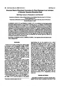
The formalism presented in section 2 is applied to liquid iron using the MD simulation technique with QJMAEAM and HZ-MAEAM. Thermodynamic states which corresponds the ionic number densities are taken from Waseda [22]. The input physical parameters of solid Fe are listed in Table 1. The model parameters calculated from input parameters and the adjustable parameters of QJ-MAEAM are given in Table 2 and Table 3 respectively. The effective interatomic pair potentials plotted at selected thermodynamic states,such as, 1833 K, 2300 K and 2900 K are shown in Figure 1 where solid and liquid indicate the results for effective potentials obtained using the lattice parameter given in the solid and liquid state.

Table 1. The input physical parameters of solid Fe.

a(A) 2.86645

Ec (eV ) 4.29

E1f (eV ) 1.79

ΩB (eV ) 12.255

ΩG (eV ) 6.555

A 2.462

Table 2. The QJ-MAEAM model potential parameters for Fe.

fe 0.395

F0 2.500

n 0.278

α 0.017

k3 0.102

k2 0.277

k1 −0.299

k0 −0.349

Table 3. The adjustable QJ-MAEAM parameters for Fe.

l3 −1.11

l2 −0.46

l1 0.95

l0 −0.24

m3 −1.14

m2 1.91

m1 −1.00

m0 0.17

0,3

Fe 1833K (liquid) 2300K 2900K 1833K (solid)

0,2

Ieff(r) (eV)

0,1

0,0 2

3

r(A)

-0,1

-0,2

-0,3

Figure 1. The effective pair potentials for liquid Fe at various temperatures.

It has noted that the pair distribution functions g(r) obtained from QJ-MAEAM with MD simulations at the corresponding thermodynamic states above melting point exhibit correct trends. Figure 2 shows the pair distribution functions calculated with both MAEAM versions. The details for HZ-MAEAM calculations can be found in elsewhere [23]. Comparing the results for QJ-MAEAM and HZ-MAEAM models with experimental data show that QJ-MAEAM model is close to experiment in both the position and height of the first peak. Although the results of g(r) for QJ-MAEAM model are shifted slightly towards smaller r values as compared with experimental data, it is observed a better agreement with experimental results than others [14]. 299

¨ ˘ S¸ENTURK DALGIC ¸ , KOC ¸ OGLU

3

QJ-MAEAM HZ-MAEAM Expt.

g(r)

2

1

0 0

4

8

12

r(A)

Figure 2. A comparison of the pair distribution functions obtained by different MAEAM models along with the experimental data.

We now turn to the thermodynamic properties of Fe. A good theory of the liquid Fe must be able to reproduce the well-established trends present in these properties. The results of our QJ-MAEAM calculations at temperature 1833K for the internal energy per atom U, the entropy per atom S and the Helmholtz free energy per atom are shown in Table 4. We also compare our MD results with those obtained using the VoterChen (VC) EAM potentials [14] and experimental values [24]. We have found that QJ-MAEAM describes well the thermodynamic properties of liquid Fe.

Table 4. The thermodynamic properties of liquid Fe.

a

MD-AMEAM VC-EAMb Expt.c a

U(eV) −3.818 −3.970 −3.520

S (10−4 eV/K) 8.512 8.973 10.432

FH (eV) −5.370 −5.610 −5.430

Present work (QJ-MAEAM),b Bhuiyan [14] , c experiment [24]

We have also obtained the diffusion coefficients with QJ-MAEAM model and plotted as a function of temperature in Figure 3. Unfortunately, experimental data for different temprature are not available for comparison with our results. The self diffusion coefficients calculated by Yokoyama using a hard sphere (HS) description are also illustrated in Figure 3 along with the results predicted by Protopapas given in Ref. [25]. It is mentioned that the computed self diffusion coefficient value of D at 1873 K is 4.40×10−7 m2 /s, that is, smaller than the values of 4.91×10−7 m2 /s and 5.46×10−7 m2 /s calculated by previous works reported in Ref.[26]. It is seen in Figure 3 that the temperature dependence of our diffusion coefficient data exhibits the Arrhenius-type behavior. However our computed values are rather slowly increasing compared with the others. Our computed values of EA and D0 are 42.27 kJ/mol and 1.58×10−7 m2 /s, respectively. These values are also more compatible with the values of 58.23 kJ/mol and 2.03×10−7 m2 /s reported in Ref. [25] than the values of 81.96 kJ/mol and 10.34×10−7 m2 /s predicted by Yokoyama [26]. 300

¨ ˘ S¸ENTURK DALGIC ¸ , KOC ¸ OGLU

-18,0

Fe A B MD

ln(D)

-18,4

-18,8

-19,2

-19,6 0,40

0,44

0,48

0,52

0,56

1000/T (K)

Figure 3. Diffusion coefficient vs. the reciprocal temperature for Fe computed by (A) Protopapas et al. [25] (B) Yokoyama [26] (MD) QJ-MAEAM.

4.

Conclusion

The structural, thermodynamic and atomic transport properties for liquid Fe have been investigated using molecular dynamics simulations in conjunction with the MAEAM potential. The basic assumption of our analysis the mechanism with the lowest self diffusion activation energy will dominate the diffusion process. The obtained results of QJ-MAEAM many-body potential for the properties of liquid Fe over wide range of temperatures are presented in this study. The simulation results are in good agreement with the available experimental values. Temperature dependence on the self-diffusion coefficient D and activation energy for liquid Fe are calculated. The presented results for thermodynamic, structure, self-diffusion properties of liquid iron show satisfactory agreement with available experimental values leads us to conclude that the molecular dynamics simulation based on QJ-MAEAM provides realistic description for liquid iron. The potentials functions of QJ-MAEAM deduced from solid-state properties give reasonable liquid properties. The discrepancy between the reported experimental diffusion coefficient and the values calculated in this work , suggested that the good reproduction of the liquid structure provides a correct value of diffusivity. For this, the M(P) term can be introduced in effective pair potential obtained from HZ-MAEAM in MD simulations. This work will be extended on this line.

References [1] M. M. G. Alemany, L. J. Gallego, L. E. Gonzalez, and D. J. Gonzalez, J. Chem. Phys., 113, (2000), 10410. [2] J. Z. Wang, M. Chen, and Z. Y. Guo, Chin. Phys. Lett., 19, (2002), 324. [3] S. Ozdemir Kart, M. Tomak, M. Uludogan, and T. Cagin, Journal of Non-Crystalline Solids, 33, (2004), 101. [4] J. I. Akhter, E. Ahmed, and M. Ahmad, Materials Chemistry and Physics, 93, (2005), 504. [5] M. S. Daw and M. I. Baskes, Phys. Rev. B, 29, (1984), 6443. [6] M. W. Finnis and J.E. Sinclair,Philos. Mag. A 50, (1984), 45. [7] R. A. Jonhson, J. Mater. Res., 3, (1988), 471.

301

¨ ˘ S¸ENTURK DALGIC ¸ , KOC ¸ OGLU

[8] R. A. Johnson, D. J. Oh, J. Mater. Res., 4, (1989), 1195. [9] B. Zhang and Y. Quyang, Phys.Rev. B, 48, (1993), 3022. [10] Y. Quyang and B. Zhang, Phys. Lett. A, 192, (1994), 79. [11] Y. Ouyang, B. Zhang, S. Liao, and Z. Jin, Z. Phys. B, 101, (1996), 161. [12] W. Y. Hu, X. Shu, and B. Zhang, Comp. Mater. Sci., 23, (2002), 175. [13] F. Fang, X. L. Shu, H. Q. Deng, W. Y. Hu, and M. Zhu, Mater. Sci. and Eng. A, 355, (2003), 357. [14] G. M. Bhuiyan, M. Silbert, and M. J. Stott, Phys.Rev. B, 53, (1996), 636. [15] S. S. Dalgic, S. Dalgic, and U. Domekeli, J. Optoelectron. Adv. Mater., 5, (2003), 1263. [16] G. Tezgor, S. S. Dalgic, and U. Domekeli, J. Optoelectron. Adv. Mater., 7, (2005), 1983. [17] S. S. Dalgic, S. Sengul, and S. Kalayci, J. Optoelectron. Adv. Mater., 7, (2005), 2001. [18] G. J. Ackland, D. J. Bacon, A. F. Calder, and T. Harry, Philos. Mag. A, 75, (1997), 713. [19] A. J. Lee, M. I. Baskes, H. Kim, and Y. K. Cho, Phys.Rev. B, 64, (2001), 184102. [20] M. I. Mendelev, S. Han,D. J. Srolovitz, G. J. Ackland, D. Y. Sun, and M. Asta, Philos. Mag., 83, (2003), 3977. [21] J. M. Haile, Molecular Dynamics Simulations, (John Wiley & Sons Inc., 1992) [22] Y. Waseda, The Structure of Non-Crystalline Materials (McGraw-Hill, New York, 1980) [23] I. Kocoglu, S. Senturk Dalgic (to be submitted). [24] R. Hultgren, Selected values of Thermodynamic Properties of Elements (American Society for Metals, Ohio, 1973). [25] T. Iida, R.I.L. Guthrie, The Physical Properties of Liquid Metals, (Clarendon Pres, Oxford,1993). [26] I. Yokoyama, Physica B, 271, (1999), 230.

302