39th IABSE Symposium – Engineering the Future September 21-23 2017, Vancouver, Canada
A monolithic approach for modeling viscoelastic materials in civil engineering Michael A. Kraus, Michael Niederwald, Geralt Siebert Contact:
[email protected]
[email protected]
Abstract This paper presents a methodology called ‘GUSTL’ [1], which is designed to efficiently estimate the parameters of a Prony-series representation of linear-viscoelastic material behaviour using measured data of the complex modulus 𝑬∗ (𝑓) obtained in a dynamic mechanical thermal analysis. ‘GUSTL’ is based on the idea of solving an inverse problem, established as a physically motivated system of linear equations, by a nonnegative least-squares procedure. The whole methodology is validated against sample data from an epoxy-coated carbon reinforcement grid for concrete structures. Keywords: viscoelasticity, material theory, Prony-series, inverse material modelling, dynamic mechanical thermal analysis (DMTA)
1
of obtaining the Prony-Series representation of a viscoelastic modulus from rate dependent data is a complex one. Usually the number of conducted tests is limited by economical and / or organizational constraints. Hence the data source for identification of the system behaviour as well as further statistical calculations such as parameter estimation is sparse. This data-sparsity introduces uncertainty in the whole estimation process. With this work we motivate a fast nonnegative least-squares solution of the model parameter estimation procedure for a Pronyseries representation of the linear-viscoelastic material behaviour when DMA data are given. The method is called ‘GUSTL’ (generalized collocation method using stiffness matrices in the context of the theory of linear viscoelasticity).
Introduction
In modern civil engineering applications many materials, such as coated carbon reinforcement grids for concrete structures or Polyvinylbutyral (PVB)-interlayers for safety glass, are polymer based. Usually these materials show strong strainrate (viscoelastic) and temperature dependent behaviour. In literature different mathematical representations (such as the hereditary integral representation or the formulation via differential equations) and measurement techniques of these phenomena exist. A very common representation is the Prony-series approach, which is implementted in many state - of - the - art Finite - Element Analysis - Software to incorporate linear viscoelastic material behaviour. The experimental determination of the Prony-series and its parameters can either be conducted via data from relaxation or retardation experiments in the time domain or from data taken under a steady state oscillation in the frequency domain, which is known as the dynamic mechanical thermal analysis. While the mathematical framework for simulating the material response for an applied excitation is straight forward, when having at hand the corresponding Prony-series for the material under investigation, the inverse problem
2
Linear Viscoelasticity
In the context of this paper only an introductory overview of the theory of linear viscoelasticity is given, further deductions and a more detailed description of the topic can be found in [3] and [4].
1
39th IABSE Symposium – Engineering the Future September 21-23 2017, Vancouver, Canada
2.1
Inspection of Figure 2 leads to the finding, that each Maxwell element almost completely decays within 2 time decades (measured in a logarithmic scale).
The Generalized Maxwell Element
The Generalized Maxwell model consists of a combination of springs and dashpots, where the combination of a single spring and a single dashpot in series is called a Maxwell element. The Generalized Maxwell Element combines K Maxwell models and one isolated spring in parallel. Thus it is a composition of K + 1 constituent elements.
Figure 2. Principal sketch of a Prony series and its individual summands, c.f. [6]
Figure 1. Generalized Maxwell Model, c.f. [1] 2.1.1
The Generalized Maxwell Element in the time domain
These basic thoughts will in chapter 4 lead to the basic structure of the method ‘GUSTL’. Finally it is introduced a more formal way of representing the Prony-series in terms of an inner product:
The total stress σ consists of two parts, the equilibrium stresses (described by the springs) and the non-equilibrium stresses (described by the dashpots): 𝐾
𝐸 𝑇 1 𝐸̂1 exp(− 𝑡⁄𝜏1 ) 𝐸(𝑡) = ( ) ⋅ ( ) =< 𝑮, 𝑩 > ⋮ ⋮ ̂ exp(− 𝑡⁄𝜏𝐾 ) 𝐸𝐾
𝐾
𝑘 𝜎 = 𝜎𝑒𝑞 + ∑ 𝜎𝑛𝑒𝑞 ⟺ 𝜎 = 𝐸𝜖 + ∑ 𝐸̂ 𝜖𝑒,𝑘 (𝑡) 𝑘=1
(1)
where the 𝐸̂𝑘 are the coordinates (summarized in the coordinate vector 𝑮) and the 𝒃𝒌 = exp(− 𝑡⁄𝜏𝑘 ) are the basis vectors (summarized in the common basis vector 𝑩).
𝑘=1
The general solution of the differential equation of the Generalized Maxwell element, Eq. (1), for arbitrary strain histories is obtained via a convolution integral (Hereditary Integral) 𝑡 𝑡 𝑡−𝑠 𝜎(𝑡) = ∫0 [𝐸 + ∑𝐾𝑘=1 𝐸̂𝑘 𝑒𝑥𝑝 (− )] 𝜖̇𝑑𝑠 = ∫0 𝑅(𝑡 − 𝑠)𝜖̇𝑑𝑠 𝜏𝑘
The time dependent relaxation properties of a material are linked to the complex moduli via the Fourier transform and vice versa:
(2)
Where 𝜏𝑖 = 𝜂𝑘 ⁄𝐸𝑘 is called relaxation time of the kth element. Special focus now shall be laid on the relaxation function 𝑅(𝑡) in eq. (2) 𝑡
̂ 𝑅(𝑡) = 𝐸 + ∑𝐾 𝑘=1 𝐸𝑘 𝑒𝑥𝑝 (− ) 𝜏𝑘
(4)
(3)
Figure 3. Structure of the Theory of Linear Viscoelasticity in the time and frequency domain, c.f. [6]
𝑅(𝑡) is called the ‘Prony-series’, which is a
composition of single decaying exponentials. A principal sketch of a Prony-series is given in Figure 2 to support the understanding of this object.
2
39th IABSE Symposium – Engineering the Future September 21-23 2017, Vancouver, Canada
2.1.2
The Generalized Maxwell Element in the frequency domain
A few important findings shall be highlighted here, further considerations can be found in [1]:
The Fourier transform of eq. (1) leads to the complex modulus E ∗ (ω): ̂ 𝑬∗ (𝜔) = 𝐸 + ∑𝐾 𝑘=1 𝐸𝑘
𝜔2 𝜏𝑘2
1+𝜔2 𝜏𝑘2
̂ + 𝑖 ∑𝐾 𝑘=1 𝐸𝑘
𝜔𝜏𝑘 1+𝜔2 𝜏𝑘2
- the storage modulus is a non-decreasing function of the frequency over the whole 𝜔 domain - if the frequency ω reaches 1⁄𝜏𝑘 , the contribution of the kth Maxwell-element to the Storage and Loss modulus is 0.5 ⋅ 𝐸𝑘
(5)
Where the real part (ℜ(E ∗ ) = 𝐸 ′ (ω)) of (5) is called the Storage modulus and the imaginary part (ℑ(E ∗ ) = 𝐸 ′′ (ω)) is called Loss modulus. Analogously to eq. (4) the complex modulus representation allows a formulation as an inner product. For the Storage and Loss modulus this reads: 𝐸 𝑇 𝐸̂ 𝐸 ′ (𝜔) = ( 1 ) ⋅ ⋮ 𝐸̂𝐾
1 𝜔2 𝜏12 1 + 𝜔 2 𝜏12 =< 𝑮, 𝑩′ > ⋮ 𝜔2 𝜏𝐾2 (1 + 𝜔 2 𝜏𝐾2 )
(6)
1 𝜔𝜏1 1 + 𝜔 2 𝜏12 =< 𝑮, 𝑩′′ > ⋮ 𝜔𝜏𝐾 (1 + 𝜔 2 𝜏𝐾2 )
(7)
𝐸 𝑇 𝐸̂ 𝐸 ′′ (𝜔) = ( 1 ) ⋅ ⋮ 𝐸̂𝐾
Figure 4. Storage Modulus basis funct. 𝒃′ 𝒌 , c.f. [1]
where the 𝐸̂𝑘 are the coordinates (summarized in 𝜔2 𝜏 2
the coordinate vector 𝑮) and the 𝒃′ 𝒌 = 1+𝜔2 𝜏𝑘2
Figure 5. Loss Modulus basis functions 𝒃′′ 𝒌 , c.f. [1]
respectively 𝒃′′ 𝒌 = 1+𝜔2𝑘𝜏2 are the basis vectors
The main behaviour of a single Maxwell-Element for the Storage modulus happens within two decades. The contribution of a single MaxwellElement is zero until one decade before its characteristic relaxation frequency 1⁄𝜏𝑘 and is constantly 𝐸𝑘 one decade after its characteristic relaxation frequency.
𝑘
𝜔𝜏
𝑘
(summarized in the common basis vector 𝑩′ and 𝑩′′). This inner product representation will be used in section 4 to define the basic regression problem, which is at the heart of ‘GUSTL’. In order to depict the frequency representation of the Prony-series, the following 5 MaxwellElements with parameters 𝜽 = [𝐸; 𝐸̂1 ; 𝜏1 ] = [0; 𝑘; 10−5−𝑘 ] with 𝑘 ∈ {1, … ,5} are considered. The Storage and Loss moduli for each of these 5 Generalized Maxwell-Elements are given in Figure 4 and Figure 5.
The main behaviour of a single Maxwell-Element for the Loss modulus happens within four decades. The contribution of a single MaxwellElement is almost zero until two decades before and two decades after its characteristic relaxation frequency 1⁄𝜏𝑘 .
A special focus shall now be again laid on the ‘influence lengths’ of the basis functions 𝒃′ 𝒌 and 𝒃′′ 𝒌 as this is the core for the later deduction of the ‘stiffness matrix’ of the ‘GUSTL’ methodology.
3
39th IABSE Symposium – Engineering the Future September 21-23 2017, Vancouver, Canada
2.2
The process of generating the ‘Master Curve’ is not a simple one despite it looks as such. A MATLAB code was developed which does a constrained spline fit on the Storage modulus curves for each measured temperature in the frequency domain and determines the horizontal shift factor 𝑎𝑇 (𝑇) as the sum of individually determined incremental shift factors 𝜕𝑎𝑇 (𝑇). For further details on the deduction and handling of this problem it is referred to [1].
Time Temperature Superposition Principle and the ‘Master Curving’ process
Typically viscoelastic material properties of polymers strongly depend on the temperature. The glass-transition temperature 𝑇𝑔 is often used as a main indicator to characterise the thermomechanical properties of polymers. The glasstransition temperature 𝑇𝑔 defines the temperature at which polymers change their state from glassy (solid) to rubbery. 𝑇𝑔 is very dependent on the chemistry of the polymer. For polymers, it is assumed, that temperature mainly changes the relaxation behaviour, thus leading to changing relaxation times (increasing temperature causes relaxation times to decrease and vice versa).
2.3
Causality and the Kramers - Kronig relation
In the context of physics and engineering causal functions are of greatest interest, as these functions respect the basic physical principle, that the effect cannot appear before the cause. Formally this is achieved by defining:
By performing short-term tests at different temperatures and shifting the measured curves on the time scale (as illustrated in Figure 6) one obtains a so called ‘Master Curve’. The ‘Master Curve’ then can be further shifted to determine the material response for any temperature of interest based on the given data set.
0 𝑡