3 State Key Laboratory for Novel Software Technology Nanjing University. Nanjing, China, 210093 ... applications as wildlife tracking for biological research and air ... history-based, which may result in a lot of miss transmission in the network ...
A Motion Tendency-based Adaptive Data Delivery Scheme for Delay Tolerant Mobile Sensor Networks 1
Fulong Xu1, Ming Liu1+, Jiannong Cao2, Guihai Chen3, Haigang Gong1, Jinqi Zhu1
Dept. of Computer Science and Engineering, University of Electronic Science and Technology of China Chengdu, China, 610054 2 Internet and Mobile Computing Lab, Department of Computing,Hong Kong Polytechnic University Hung Hom, Kowloon, Hong Kong 3 State Key Laboratory for Novel Software Technology Nanjing University Nanjing, China, 210093
Abstract—The Delay Tolerant Mobile Sensor Network (DTMSN) is a new type of sensor network for pervasive information gathering. Although similar to conventional sensor networks in hardware components, DTMSN owns some unique characteristics such as sensor mobility, intermittent connectivity, etc. Therefore, traditional data gathering methods can not be applied to DTMSN. In this paper, we propose an efficient Motion Tendency-based Data Delivery Scheme (MTAD) tailored for DTMSN. By using sink broadcast instead of GPS, MTAD obtains the information about the nodal motion tendency with small overhead. The information can then be used to evaluate the node’s effective delivery ability and provide guidance for message transmission. MTAD also employs the message survival time to effectively manage message queues. Our simulation results show that, compared with other DTMSN data delivering approaches, MTAD achieves not only a relatively longer network lifetime but also a higher message delivery ratio with lower transmission overhead and data delivery delay. Keywords-DTMSN; data gathering; queue management
I.
INTRODUCTION
Advances in wireless communications and integrated circuits have enabled the development of small and inexpensive wireless sensor devices. A large number of these cheap sensor nodes can be networked together and form wireless sensor networks (WSNs). Data gathering is one of the major functions of WSNs. The data gathering approaches in the traditional WSNs usually rely on a large number of densely deployed sensor nodes with short range radio to form a well connected end-to-end network. Sensor nodes in the network collaborate with each other to collect the target data information and transmit them to the sink nodes [1]. Although these approaches are well suited to many data gathering applications, they cannot work effectively to deal with such applications as wildlife tracking for biological research and air quality monitoring, which experience extremely low and intermittent connectivity due to sparse network density and sensor nodes mobility. As an application of Delay-Tolerant Network (DTN) [2] on sensor networks, Delay Tolerant Mobile Sensor Network (DTMSN) [3] has been proposed in recent years to address the aforementioned problem. A typical DTMSN consists of two
types of nodes, the mobile sensor nodes and some sink nodes. The former are attached to some mobile objects, gathering target information and forming a loosely connected mobile sensor network for information delivery. The sink nodes in DTMSN are either deployed at special locations or carried by a subset of mobile objects to receive data from sensors and forward them to access points of the backbone network. Since the connectivity between mobile sensors is poor, it is difficult to form a well connected end-to-end network for data transmission. In order to achieve certain successful delivery ratio in such an opportunistic network, data replication is necessary. However, multiple copies of messages will increase transmission overhead, which is a substantial disadvantage for energy limited sensor networks. Therefore, how to achieve the tradeoff between the data delivery ratio/delay and the delivery overhead is a key research issue in DTMSN. Different techniques have been proposed for data gathering in DTMSN [4]. One strategy is that data delivery is allowed only when sensors are in the proximity of the sinks. Although it has very little communication overhead, the delivery delay could be very long. Another strategy is to employ epidemic to increase the delivery ratio. However, since too many message copies are produced, this strategy may cause large communication overhead. In [5] the authors proposed a delivery-probability based routing protocol. However, the method for calculating the delivery probability is entirely history-based, which may result in a lot of miss transmission in the network, causing adverse effects on its performance. In this paper, we propose MTAD, a Motion Tendencybased Adaptive data Delivery scheme. MTAD achieves a good performance by replicating messages and sending them to the nodes with higher probability of meeting the sink. Different from the existing protocols, MTAD uses the sink broadcast instead of GPS, to make the sensor node be aware of its motion tendency. Then through the movement prediction, the node’s effective delivery capability is evaluated and used for the guidance of message transmission. In addition, MTAD employs message survival time to indicate the importance of a message and to decide whether a message should be transmitted or dropped for minimizing the transmission overhead. We evaluate the effectiveness of MTAD by simulations and compare its performance with three popular
978-1-4244-4148-8/09/$25.00 ©2009 This full text paper was peer reviewed at the direction of IEEE Communications Society subject matter experts for publication in the IEEE "GLOBECOM" 2009 proceedings.
existing DTMSN routing protocols, namely direct transmission, flooding and FAD. Simulation results show that, compared with the three protocols, MTAD achieves a longer network lifetime and higher message delivery ratio with lower transmission overhead and data delivery delay. The rest of the paper is organized as follows: Sec. II discusses related works. Sec. III discusses the motivation and the mobility model used in our paper. Sec. IV introduces MTAD. Sec. V shows the effectiveness of MTAD via simulation. Sec. VI concludes the paper. II.
utilization. In [10], the authors propose a FAD protocol to increase the data delivery ratio in DTMSN. Besides using the same delivery probability calculation method as RED, FAD further discusses how the replication of the data over the sensor network can be constrained using a fault tolerance value associated to each data message. As mentioned above, due to the ineffective delivery probability calculation technique used for the choice of the nodes as next hop, that protocol still has quite a high overhead. III.
RELATED WORK
Various approaches have been proposed to address the data gathering problem in DTMSN. The most basic and simple protocol is direct transmission [5], where data would be to only allow delivering when sensors are in direct proximity of the sinks. Although this protocol has very little communication overhead, the delivery of the data is poor and the delivery ratio might be very low, because in DTMSN scenario the sensor nodes can not meet the sink nodes frequently. Another basic protocol is flooding protocol [6], where a sensor always broadcasts the data messages in its buffer to all the nearby sensors, which receive the data messages, keep them in the buffer queue, and rebroadcast them. If the queue is large enough, the flooding protocol could achieve a low data delivery delay and high delivery ratio at the cost of more traffic overhead and energy consumption. However, the buffer size of sensor is usually limited, which results in many message dropping and retransmission in flooding. In order to learn zebras’ behavior, the ZebraNet project [7] proposes a history-based approach for routing. The routing decision here is made according to a sensor’s past success rate of transmitting data packets to the sink nodes directly. The Shared Wireless Info-Station (SWIM) system is proposed in [8] for gathering information of radio-tagged whales, assuming the randomly moving of sensors have the same probability of meeting the sink, and thus a sensor node needs only to distribute a number of copies of packet to other nodes so as to attain the desired data delivery ratio. However, in practical scenarios, different nodes may have different probabilities of meeting the sink, so SWIM can not work efficiently. Other endeavors aiming to enhance the performance of DTMSN routing include paper [9, 10, 11]. In [9], a replication based efficient data delivery (RED) protocol is presented. RED uses a history-based method like ZebraNet to calculate the delivery probabilities of sensor nodes. When message transmission occurs, the delivery probability of the source sensor increases; contrarily if there is no transmission during a given interval, the delivery probability would decrease. However, in DTMSN scenarios where nodes are sparse and intermittently connected, it often takes a comparatively long time for a node to meet another which has a higher delivery probability. Therefore the updating frequency of the delivery probability in RED is usually low, and there may exist sensors which are far away from the sink but still have high delivery probabilities. Thus the history-based method is not effective and cannot denote the actual ability that a node delivers data to sink nodes. In addition, the message management of propagating many small messages in the network may incur further processing overhead and inefficiency of bandwidth
NETWORK MODEL AND PROBLEM STATEMENT
A. Network Model We assume initially all the sensor nodes are randomly deployed in a square area with size M×M, and the only static sink node is located at the center of this area. All the sensor nodes have the same maximum transmission range R. Moreover, we further assume some additional characteristic of our sensor network. •
The mobility of all sensor nodes is assumed to follow the Random Waypoint (RWP) model [12].
•
The only static sink node is deployed as a base station, thus the energy of the sink can be regarded as infinite.
•
The transmit power of sink nodes is variable. By varying its transmit power, a sink can control its transmission range elastically.
The first item described above prescribes the sensor nodes’ moving pattern. As a typical mobility model, RWP is widely used in the research of mobile wireless networks. The second assumption about the sink node is considered reasonable and acceptable for practical application. As for the assumption about the controllable transmit power, it enables the sink to broadcast with a wide range of coverage. B. Problem Statement DTMSN distinguishes itself from conventional WSNs by the following unique characteristics: 1) Nodal mobility. Since the sensor nodes are attached to randomly moving objects, the network topology is highly dynamic; 2) Intermittent connectivity. Intermittent connectivity is caused by the dynamic network topology; 3) Sparse density. Node density is normally much lower in DTMSN compared with the traditional densely deployed sensor networks, which further deteriorates the network connectivity; 4) Delay tolerable. Data delivery delay in DTMSN is high. Such delay, however, is usually tolerable in the applications. According to these characteristics, an efficient DTMSN data delivery scheme must adaptively select the nodes that are more likely to meet the sink node as the next hop. Furthermore, since data messages may be stored in the buffer queue for quite a long time before being transmitted, proper queue management is another challenge for effective data delivering. IV.
THE PROPOSED MOTION TENDENCY-BASED DATA DELIVERY SCHEME
In this section, we present a novel data gathering protocol MTAD, which aims to attain a high data delivery ratio with
978-1-4244-4148-8/09/$25.00 ©2009 This full text paper was peer reviewed at the direction of IEEE Communications Society subject matter experts for publication in the IEEE "GLOBECOM" 2009 proceedings.
low data delivery overhead/delay by using motion prediction. MTAD consists of two components: data transmission and queue management. A. Data Transmission Data transmission decision is made based on the delivery probability, which indicates the likelihood that a sensor node communicates with the sink. Intuitively, a sensor’s delivery probability is associated with the relative distance between itself and the sink node. The closer this distance is, the better delivery ability the sensor has. Moreover, due to the mobile characteristic of the sensor node, the delivery probability is also related to the sensor’s moving speed and direction. Therefore, by judging a sensor node’s move tendency we can determine its data delivery probability. 1) Acquire information about nodal motion tendency We first introduce a simple method making a sensor node be aware of its relative distance to the sink. Although using GPS or directional antennas is a common solution to detect location, attaching these equipments to sensor nodes not only increases the cost but also aggravates nodal energy consumption. With no GPS, in our scheme the sink node broadcasts a beacon message with the high transmit power periodically (e.g., once every 5 seconds). As the beacon message size is small, the impact of the broadcasting on the network performance is quite weak. We will demonstrate it in section V. Based on the high-level transmit power, the broadcast range of coverage is broad enough to cover most of the sensors. Since the signal attenuation of the broadcasting is associated with its transmission distance, the closer a sensor is to the sink, the stronger signal strength it will perceive, thus the continual perceived signal strength of beacon messages could then be used to evaluate how far it is to the sink. More specifically, when a sensor node receives the beacon message, it perceives the signal strength, calculates the current relative distance and records it in a list. Now we learn and evaluate one sensor’s motion tendency by trigonometry. Without loss of generality, we consider a sensor i. Fig.1 is the schematic view about this sensor’s movement, and we assume it is moving straight at a speed v. The larger gray node S in Fig.1 denotes the sink node, and the point C denotes the momentary position of sensor i when the current sink broadcast occurs. The point P, from which an arrow line is drawn toward C, is the previous position of sensor i receiving the beacon message the last time. Assuming the sensor would still keep moving for a while, during a following specific time τ, the sensor i could move from C to the predictive location N. The length of line CN is denoted by Lcn (the lengths of other line segments have the similar expression). It’s easy to find that
Lcn = vτ
L pc = vω ,
(1) (2)
where Lpc is the length of line PC and ω is the sink broadcast interval. As the lengths of the other two lines SP and SC (expressed by Lsp and Lsc) are just the relative distances already acquired through sink broadcast, using simple trigonometry we get formulas as follows:
α = π − arccos(
L pc 2 + Lsc 2 − L sp 2
)
(3)
Lsn = Lsc 2 + Lcn 2 − 2 Lsc Lcn cos α
(4)
Lcn 2 + L sn 2 − Lsc 2 ). 2 Lcn Lsn
(5)
β = arccos(
2 L pc L sc
P P’
C α
P θ
N β S(sink)
C
S(sink)
Fig.1. The motion prediction of sensor node i
Fig.2. Using the distance from the sink to calculate motion speed
From formulas (1)-(5) we can find that, so long as the speed v is known, the value of α, Lsn and β could be figured out successively. These three variables, as important characterization of the predictive location N, will be used to evaluate sensor i’s delivery ability. We will describe it at the next subsection. Although it seems difficult for a moving sensor node to sense its speed, fortunately, there is a simply method to calculate it. Considering sensor i is moving straight with speed v, as shown in Fig.2, when the latest three broadcasting occur, the momentary positions of sensor i are respectively at P’, P and C. Using trigonometry we get formulas as follows:
L p ' p = L pc = vω
θ = π − arccos(
cos θ =
(6)
L p ' p 2 + Lsp 2 − Lsp ' 2 2 L p ' p Lsp
L sp 2 + L pc 2 − Lsc 2 2 L sp L pc
)
.
(7)
(8)
According to formulas (6)-(8) we can deduce the speed:
v=
Lsp ' 2 + Lsc 2 − 2 L sp 2 2ω 2
.
(9)
From formula (9) we find that the speed v is associated with the three variables Lsp’,Lsc and Lsp. All of them can be acquired through broadcast. Thus, so long as the duration of the motion is longer than 3ω (at least 2ω), the sensor’s speed could be figured out by itself. This is practicable since the 3ω is generally a very short time. Furthermore, before the concrete speed can be calculated, an approximate estimate speed value could be used to get a rough Pi if needed.
2) Calculate Data Delivery Probability The process of calculating Pi can be categorized into the following three cases, according to the predictive location N:
978-1-4244-4148-8/09/$25.00 ©2009 This full text paper was peer reviewed at the direction of IEEE Communications Society subject matter experts for publication in the IEEE "GLOBECOM" 2009 proceedings.
a) If the sensor i is just within the communication range of the sink node, no matter what the motion is, Pi is set to 1. Because sensor i can directly communicate with the sink now. b) If the sensor’s current moving path from point C to the predictive N intersects the communication range of the sink node, then Pi is set to 1. Since the node is moving towards the sink node and will communicate directly with it soon. C α β
N
S Fig.3. Sketch map of the moving path crossing the communication range of sink
As shown in Fig.3, in such a case the angles α and β are both acute, and the distance from the sink node to the path line is shorter than R. The following group of formula could be the judgment of this case. It is simple so we omit its proof here. ⎧ cosα cos β > 0 ⎨ ⎩ L sc sin α ≤ R.
(10)
c) If the above two cases can not be hold, then according to the network model, sensor i is moving forward and will probably appear at position N during the time τ. We make decision on calculating Pi according to the distance between N and the sink node. The formula is described below: ⎧ R , ⎪ Pi = ⎨ L sn ⎪⎩ 1,
Lsn > R
(11)
L sn ≤ R.
The formula (11) means that if the location N is within the communication range of the sink, Pi is set to 1; otherwise Pi is inversely proportional to Lsn. Therefore, for one sensor moving toward the sink node, its delivery probability increases gradually, while moving apart, decreases. 3) Data transmission algorithm Data transmission decision is made based on the delivery probability. We also consider the sensor i, which has a total number of n messages in the data queue ready for transmission and is moving into the communication range of a set of Z’ sensors. Let Σ={Ψz︱1≤z≤ Z’} represent the Z’ nodes. Sensor i first learns their current delivery probabilities via simple handshaking messages and then replicates all the messages in its queue to a subset of the Z’ sensors, which have higher delivery probabilities than Pi. B. Queue management The goal of the queue management is to determine message’s transmission order in the buffer queue and which data message should be dropped when the queue is full. The main idea of our queue management is to employ the message survival time to signify the importance of a given message. 1) Message survival time We assume each data message has a field to record its
survival time. When a message is generated, its survival time is initialized to be zero. In order to update the survival time, each sensor maintains a timer. Once the timer expires, all the stored messages’ survival time are increased. Let’s consider a message which is being replicated between two sensors, since the propagation time between two adjacent nodes with short distance can be ignored, thus the receiver would insert the message to its own queue directly without any modification to the survival time. As far as the source message which is inserted into source node’s queue again after being transmitted to its next hop, its survival time also remains unchanged. 2) The implementation of queue management scheme Each sensor has a data queue that contains data messages coming from three sources. (a) when the sensor acquires data from its sensing unit, it creates a data message and inserts it into the queue; (b) When the sensor receives a data message from other sensors, the message is inserted into the data queue; (c) After the sensor sends out a data message to a non-sink node, it may insert the message again if the message is created by the source sensor node itself, because the message is not guaranteed to be delivered to the sink node. We believe that the message with smaller survival time is more important and should be transmitted with a higher priority. This is embodied by arranging the messages in the queue with an increasing order of their survival time. A message will be dropped at the following two occasions. First, if the queue is full when a message arrives, the oldest one among all the messages (including the new coming one) is dropped. Second, once the survival time of a message in the process of updating exceeds the network’s delay tolerant threshold (the maximum delay value of message), the message is dropped. This is to reduce network energy consumption, given that the message either has been delivered to the sink node with a high probability by other sensors or has been invalid in our application. V.
SIMULATION
In this section, we simulate and evaluate four protocols: the proposed MTAD, FAD, direct transmission and the flooding. A. Simulation Environment In our experimental environment, we assume the data generation of each sensor follows a poisson process with an average arrival interval of 100 s. The default sink broadcast interval of MTAD is 5 s, and the broadcast radius is 100 m. To evaluate the network lifetime, we use the same radio energy dissipation model as in [13]. Other simulation parameters and their default values are summarized in Table 1. In particular, for the flooding protocol, after the queue is full, only the messages newly generated by the node itself are allowed into the queue, no longer accepting the messages transmitted from other sensors. All the simulation results are averaged over 1000 independent runs. B. Performance Comparison We first compare the performance of the four schemes under the default parameters, and the results are shown in Table 2. As we can see, compared with other three protocols, the MTAD method achieves the highest delivery ratio with lower transmission overhead (indicated by the average copies
978-1-4244-4148-8/09/$25.00 ©2009 This full text paper was peer reviewed at the direction of IEEE Communications Society subject matter experts for publication in the IEEE "GLOBECOM" 2009 proceedings.
for each message) and the lowest average delivery delay. The direct transmission protocol performs worst in terms of delivery ratio and average delay, because the sensor nodes can only transmit messages to the sink node directly. It’s ineffective for message delivery as in DTMSN a sensor meet the sink infrequently. Moreover, we find that for the flooding protocol, its delivery ratio is a little higher and the average delivery delay is slightly lower than the direct transmission. This is due to the special queue management of flooding, where only the newcome messages generated by the sensor itself are allowed into the queue after the queue is full. Consequently, the messages in the queue can be divided into two types, messages copies created by flooding and single data messages coming later. The former can be delivered to the sink node through different sensor nodes (flooding effect) while the latter can only be delivered by the source node. As a result, the overall delivery ratio and average delay of the flooding protocol outperforms the direct transmission. From Table 2 we also find that the FAD method performs worse comparing with MTAD, especially in term of transmission overhead. As mentioned above, the history-based delivery probability calculation method of FAD is not effective, and the miss transmission causes messages to be relayed more times before reach the sink node. In contrast, the MTAD is more accurate in the selection of the next hop, and its simple queue scheme, cooperating with this delivery probability method, effectively deals with the tradeoff between data delivery ratio/delay and overhead. Table1. Simulation parameters Parameter Network size (m) Number of sensor node Transmission radii R(m) Sink broadcast interval ω (s) High power-level transmission radii of sink (m) Prediction time τ (s)
Speed of sensor node V(m/s) Pause time Tpause (s) Maximum queue size of sensor Size of data message Size of broadcast message Message generation rate Position of sink node Maximum delay tolerant value(s) Fault tolerance threshold of FAD α of FAD Timer expiration value Δ of FAD Initial energy of sensor node (joule)
Default Value 200×200 100 3 5 100 6 1~5 0~120 200 messages 200 bits 20 bits 0.01/s (100, 100) 2000 0.9 0.1 30 10
Table.2 Simulation results with default parameters
Delivery ratio (%) Average copies for each message Average delay(s)
MTAD
FAD
91.5
85.8
Direct Transmission 61.6
3.2
7.0
1.0
9.6
346.6
396.4
1646.5
1454.2
Flooding 68.9
C. Impact of Nodal Transmission Range We also vary the transmission range of each sensor in our simulations, with results presented at Fig 4. As expected, the MTAD approach always has a higher delivery ratio than others, except when the transmission radii is 1 m (with the very
small transmission radii of 1 m, the queue scheme which cause more duplications acquires the high delivery ratio). With the increase in transmission range, the delivery ratio increases for all approaches because the sensors have higher probabilities of meeting others, increasing the probability of message relaying. In particular, for FAD there is sharp decrease in both delivery ratio and average copies when the transmission range is larger than 7 m. It’s because that with the big transmission range, the common interval that one sensor encounters neighbors who have higher delivery probabilities is shorter than the default Δ of FAD (as a rule of FAD, if there is no message transmission within the interval of Δ, the sensor’s delivery probability is reduced). Therefore, most sensors’ delivery probabilities would always increasing and become improperly big. As the fault tolerance scheme of FAD is based on the delivery probability, with the unreasonable high delivery probabilities, messages would be discarded more easily when being transmitted, thus both the delivery ratio and the number of average copies decrease. Fig. 4(b) shows that, except the direct transmission, the number of average copies of other protocols increase with the transmission range. Fig. 4(c) demonstrates that the average delay of each protocol decreases when transmission range becomes large. D. Interference of Sink Broadcasting As sensors and the sink share the common radio channel, the sink broadcast would interfere with the normal message transmissions between sensors. When the broadcasting occurs, all the ongoing transmissions of which the receiving nodes are covered in the broadcast range are interfered and would be relaunched later, resulting in additional overhead. Now we evaluate the impact of the sink broadcast. With the default simulation parameters we find that, the amount of the transmissions interfered by broadcasting is just 0.47% of total transmissions during the whole network lifetime. Fig. 5 illustrates the impact of different broadcast interval on the interference ratio. As expected, with the decrease of the broadcast interval, the interfered transmission increases. However, even if the broadcast interval is 1 s, the interference ratio is only 2%. Fig. 6 shows the impact of different broadcast radii on the interference ratio, and we find that even if the broadcast radius is 150 m and thus the whole area is covered, the corresponding interference ratio is only 0.53%. There are two reasons for the inappreciable impact of the broadcast interference. First, the beacon message size is very small. Despite of the wide broadcast range, the transmission is very fast. Second, as the low and intermittent connectivity in the network, the simultaneous transmission is infrequent, which also weaken the broadcast impact. E. Network life analyze Table 3 Network life with default parameters
Network lifetime(day)
MTAD
FAD
Flooding
Direct Transmission
7.57
4.29
46
1155
Having a long network life is very important for DTMSN, because the sensor nodes in the network are generally energyconstrained. We assume the network ends up when half of the sensor nodes exhaust their energy. The simulation results are
978-1-4244-4148-8/09/$25.00 ©2009 This full text paper was peer reviewed at the direction of IEEE Communications Society subject matter experts for publication in the IEEE "GLOBECOM" 2009 proceedings.
60 FAD MTAD Direct Flood
Average copies
Delivery ratio(%)
50
FAD MTAD Direct Flood
40
Average delay(s)
100 90 80 70 60 50 40 30 20 10 0
30 20 10 0
1
2
3 4 5 6 7 8 Transmission radii R(m)
9
1
10
2
3 4 5 6 7 8 Transmission radii R(m)
9
10
(b)Average copies
(a)Average delivery ratio
2200 2000 1800 1600 1400 1200 1000 800 600 400 200 0
FAD MTAD Direct Flood
1
2
3 4 5 6 7 8 Transmission radii R(m)
9
10
(c)Average delay
Fig.4. Impact of Nodal Transmission Range
2.5
0.6
2
0.5
Interfere ratio (%)
Interfere ratio (%)
presented in table 3. As expected, the direct transmission protocol achieves the longest network lifetime. The flooding protocol attains a comparatively long lifetime in our simulation. It’s still caused by the special queue scheme. During the initial flooding time, great duplication consumes energy rapidly until most queues are full. After that, message exchange between sensors is infrequent, and energy consumption decreases. Another simulation is also done with a queue size of 3000 messages, and the network lifetime decreases sharply to 1 day because the larger queue extends the flooding phase. We also find that the MTAD protocol gains a longer lifetime which is almost twice lifetime the FAD attains. Although receiving broadcast messages consumes energy, this consumption is teeny as the beacon message size is very small. Simulations confirm that in MTAD, through one sensor’s whole lifetime, the energy spent on broadcast receiving is only 1.1% of the total. Thus the impact of the broadcast is weak on the network lifetime, and the lifetime mainly depends on the effectiveness of the data delivery scheme.
1.5 1 0.5 0
Foundation of China under Grants No.60703114, 60573131, 60825205; under CERG grant PolyU 5102/07E, Hong Kong Polytechnic Univ. under ICRG grant G-YF61; the Youth Teacher Foundation of UESTC under Grants L08010601JX0746, L08010601JX0747. REFERENCES [1]
[2]
[3]
[4]
[5]
[6]
0.4
[7]
0.3 0.2
[8]
0.1 0
1
2
3
4
5
6
Broadcast interval (s) Fig.5. Broadcast interval vs Interfere ratio
VI.
7
25
50
75
100
125
Broadcast radii R(m) Fig.6. Broadcast radii vs Interfere ratio
150
[9]
CONCLUSION
This paper first introduces the unique characteristics of DTMSN, such as sensor mobility, loose connectivity, and delay tolerability. Based on these characteristics, we have proposed a non-GPS motion tendency-based adaptive data delivery scheme. Simulations have been carried out for performance evaluation. The results show that, comparing with other DTMSN data delivering approaches, the proposed MTAD protocol achieves a higher message delivery ratio with lower delay and transmission overhead.
[10]
ACKNOWLEDGE
[13]
This work is supported by the National Natural Science
[11]
[12]
I Akyildiz, W Su, and Y Sankarasubramania, “A survey on sensor networks,” IEEE Communications Magazine, vol.40, pp. 102-114, 2002. K Fall, “A delay-tolerant network architecture for challenged internets,” In Proceedings of ACM SIGCOMM 2003 Conference on Computer Communications. 2003, pp. 27-34. Y. Wang, F. Lin, and H. Wu,“Poster: Efficient Data Transmission in Delay Fault Tolerant Mobile Sensor Networks (DFT-MSN),” Proceedings of IEEE International Conference on Network Protocols (ICNP’05), 2005. Y Wang, H Dang, H Wu. “A survey on analytic studies of DelayTolerant Mobile Sensor Networks.” Published online in Wiley InterScience (www.interscience.wiley.com), vol.7,pp.1197-1208. 2007 Y Wang and H Wu, “Delay/Fault-Tolerant Mobile Sensor Network (DFT-MSN): a new paradigm for pervasive information gathering,” IEEE Transactions on Mobile Computing, vol. 6, pp. 1021-1034,2006. Vahdat A and Becker D, “ Epidemic routing for partially connected ad hoc networks,” Technical Report CS-200006, Duke University, 2000. Philo J, Hidekazu O, and Yong w, “Energy-efficient computing for wildlife tracking: design tradeoffs and early experiences with ZebraNet.,” ACM Operating System Review, vol. 36, pp,:96-107, 2003. T Small and Z J Haas, “The shared wireless infostation model – a new Ad Hoc networking paradigm (or where there is a whale, there is a Way),” In Proceedings of ACM International Symposium on Mobile Ad Hoc Networking and Computing (MOBIHOC’03). 2003, pp. 233-244. Y Wang and H Y Wu, “Replication-Based efficient data delivery scheme (RED) for Delay/Fault-Tolerant mobile sensor network (DFTMSN),” In Proc. Of Fourth Annual IEEE International Conference on Pervasive Computing and Communications Workshops, 2006, pp. 485489. Y.Wang, H.Wu, H.Dang, and F.Lin, “Analytic,Simulation, and Empirical Evaluation of Delay/Fault-Tolerant Mobile Sensor Networks,” IEEE Transactions on Wireless Communications. 2007,pp. 3287-3296. Y.Wang and H Y Wu, “Dft-msn: The delay fault tolerant mobile sensor network for pervasive information gathering,” In Proc. of Twenty-Fifth Annual Joint Conference of the IEEE Computer and Communications Societies (INFOCOM), 2006 Camp T, Boleng J, and Davies V, “ A survey of mobility models for ad hoc network research,”Wireless Communication and Mobile Computing, vol.2, pp. 483-502, 2002. Heinzelman WR., “An application-specific protocol architecture for wireless microsensor networks.,” IEEE Trans. on Wireless Communications, vol.1, pp. 660−670, 2002.
978-1-4244-4148-8/09/$25.00 ©2009 This full text paper was peer reviewed at the direction of IEEE Communications Society subject matter experts for publication in the IEEE "GLOBECOM" 2009 proceedings.