A MOVING PSEUDO-BOUNDARY MFS FOR VOID DETECTION IN TWO-DIMENSIONAL THERMOELASTICITY A. KARAGEORGHIS, D. LESNIC, AND L. MARIN
Abstract. We investigate the numerical reconstruction of smooth star-shaped voids contained in a two-dimensional isotropic linear thermoelastic material from the knowledge a single non-destructive measurement of the temperature field and both the displacement and traction vectors (over-specified boundary data) on the outer boundary. The primary fields, namely the temperature and the displacement vector, which satisfy the thermo-mechanical equilibrium equations of linear thermoelasticity, are approximated using the method of fundamental solutions (MFS) in conjunction with a two-dimensional particular solution proposed in [37]. The fictitious source points are located both outside the (known) exterior boundary of the body and inside the (unknown) void. The inverse geometric problem reduces to finding the minimum of a nonlinear least-squares functional that measures the gap between the given and computed data, penalized with respect to both the MFS constants and the derivative of the radial polar coordinates describing the position of the star-shaped void. The interior source points are anchored to and move with the void during the iterative reconstruction procedure. The stability of the numerical method is investigated by inverting measurements contaminated with noise.
1. Introduction Numerous problems in solid mechanics are characterised by the fact that at least one of the following conditions is entirely or partially unknown: (i) the governing partial differential equations; (ii) the geometry of the domain of interest; (iii) the material properties; and (iv) the boundary and initial conditions. Such problems are called inverse problems. Most of them are ill-posed and, consequently, are more difficult to solve than direct problems. It is also-well known that inverse problems are in general ill-posed in the sense of Hadamard [15], meaning that small errors in the boundary and or initial data may significantly amplify the errors in the solution. Inverse geometric problems represent an important subclass of inverse problems and are characterised by a partial knowledge of the geometry of the solution domain, i.e. condition (ii) is incompletely known, whilst the remaining conditions (i), (iii) and (iv) are all known. In these problems, it is generally assumed that only a part of the boundary of the solution domain is known and accessible, while the remaining boundary is unknown and unaccessible and has to be determined from additional boundary data available on the accessible and known portion of the boundary or some internal measurements. In this study we refer to applications in the non-destructive evaluation of two-dimensional voids (e.g. rigid inclusions and cavities) in steady-state linear isotropic thermoelastic solids, for which the boundary temperature, displacements and tractions are measured on the accessible exposed surface, the boundary condition on the void surface is known, while the geometry of the void is to be determined. The large majority of the theoretical and numerical studies devoted to the non-destructive detection of cavities and/or inclusions embedded in an elastic material available in the literature have considered either thermal [3, 5, 11, 12, 16, 18, 19, 21, 22, 25, 27, 28, 33, 39] or mechanical data [1, 2, 6, 7, 9, 17, 22, 24, 35, 38, 43, 44] measured on the accessible boundary and the corresponding boundary conditions on the unknown cavity/inclusion, i.e. either the heat conduction equation in isotropic solids or the equilibrium equations for isotropic linear elastic bodies have been considered. At the same time, to the best of our knowledge, there are only a few studies available in the Date: September 20, 2013. 2000 Mathematics Subject Classification. Primary 65N35; Secondary 65N21, 65N38. Key words and phrases. Void detection, inverse problem, method of fundamental solutions, thermoelasticity.
1
2
A. KARAGEORGHIS, D. LESNIC, AND L. MARIN
literature that deal with the theoretical and/or numerical reconstruction of voids in an isotropic linear thermoelastic material, i.e. by measuring the thermo-mechanical fields at boundary and/or internal points [8, 10, 29, 30]. The method of fundamental solutions (MFS) [13, 14] is a meshless boundary collocation method [32] which may be used for the numerical solution of certain boundary value problems. This method, originally proposed in the mid 60s by Kupradze and Aleksidze [34] and introduced as a numerical method in the late 70s by Mathon and Johnston [41], has become increasingly popular primarily because of the ease with which it can be implemented. Due to this latter feature and the ideal suitability of the method for problems in which the shape of the boundary needs to be determined as part of the solution, the MFS has been used extensively for the numerical solution of inverse and related problems in the last decade. An extensive survey of applications of the MFS to inverse problems is provided in [23]. It should be mentioned that the MFS was used for the first time for the solution of inverse geometric problems in linear elasticity in [6], where the method of Kirsch and Kress [31] (originally proposed in the context of an exterior acoustic scattering problem) was adapted to the detection of rigid inclusions or cavities in an elastic body. The method of Alves and Martins [6] decomposes the inverse problem into a linear and ill-posed part in which a Cauchy problem is solved using the MFS, and a nonlinear part in which the unknown boundary of the void is sought as a zero level set for a rigid inclusion (or computed iteratively, in an optimization scheme for a class of approximating shapes, for a cavity). In contrast, in this paper we adopt a fully nonlinear MFS in which the nonlinear and ill-posed parts are dealt with simultaneously using a nonlinear regularized minimization. Moreover, in the method adopted herein the interior source points are free to move during the reconstruction procedure which is a further novel feature compared with earlier approaches. Encouraged by the recent results obtained using the MFS for the detection of rigid inclusions and cavities (i.e. inner boundaries with prescribed homogeneous Dirichlet and Neumann boundary conditions, respectively) from Cauchy data measured on the outer boundary in the two- and three-dimensional Laplace equation [11, 21, 25] and the Lamé system in planar (two-dimensional) elasticity [24], we extend the MFS to the numerical reconstruction of voids in two-dimensional isotropic linear thermoelasticity. The paper is organized as follows. In Section 2, the inverse geometric problem considered herein is formulated mathematically. Section 3 is devoted to the MFS approximation for the aforementioned inverse problem via the MFS particular solution for the planar thermoelasticity system proposed in [37]. Implementational details on the penalized least-squares functional and the regularization method employed are given in Section 4. Four numerical examples associated with the numerical detection of a single void in planar thermoelasticity are thoroughly investigated in Section 5 and, furthermore, the proposed method is extended and applied to the numerical reconstruction of multiple voids in Section 6. Finally, some comments, conclusions and future related work are given in Section 7. 2. Mathematical Formulation Consider a two-dimensional annular domain Ω = Ω2 \ Ω1 , where Ω1 ⊂ Ω2 , and Ω1 , Ω2 are open bounded and simply-connected domains bounded by the interior and exterior smooth boundaries ∂Ω1 and ∂Ω2 , respectively, see Figure 1. We further assume that Ω is occupied by an isotropic solid characterised by the thermal conductivity, κ, the coefficient of linear thermal expansion, αT , Poisson’s ratio, ν, and the shear modulus, G. In the framework of isotropic linear thermoelasticity, under the assumption of small displacements the stress tensor σ = [σij ]1≤i,j≤2 is related to the displacement vector u = (u1 , u2 ) by means of the constitutive law of thermoelasticity [ ] ( ) ) 2ν ( σ(x) = G ∇u(x) + ∇u(x)T + (2.1) ∇ · u(x) I − γ T (x) I , x = (x1 , x2 ) ∈ Ω . 1 − 2ν / In (2.1), ν/= ν for a plane strain state and ν = ν (1 + ν) for a plane stress state, while αT/ = αT and αT = αT (1 + ν) (1 + 2ν) for the plane strain and plane stress states, respectively, γ = 2G αT (1 + ν) (1 − 2ν) and I is the 2 × 2 identity matrix.
MOVING MFS FOR VOID DETECTION
3
In the absence of body forces, one obtains the equilibrium equations of two-dimensional isotropic linear static thermoelasticity in terms of the displacement vector and the temperature (also known as the Navier-Lamé system of two-dimensional isotropic linear thermoelasticity), namely 0 = −∇ · σ(x) = L u(x) + γ ∇T (x),
x ∈ Ω,
(2.2)
T
where L = (L1 , L2 ) is the partial differential operator associated with the Navier-Lamé system of isotropic linear elasticity, i.e. [ ] ) ( ( ) 2ν T L u(x) ≡ −G ∇ · ∇u(x) + ∇u(x) + ∇ ∇ · u(x) , x ∈ Ω . (2.3) 1 − 2ν ( )T Further, we let n(x) = n1 (x), n2 (x) be the outward unit normal vector at ∂Ω and t(x) be the traction vector at x ∈ ∂Ω given by t(x) = σ(x) n(x) , x ∈ ∂Ω . (2.4) On the outer boundary ∂Ω2 we prescribe both the displacement and traction vectors, i.e. x ∈ ∂Ω2 .
(2.5a)
t(x) = g 2 (x) , x ∈ ∂Ω2 . On the inner boundary, we have boundary conditions in the form
(2.5b)
u(x) = f 2 (x),
Λ u(x) + (I − Λ) t(x) = Λ f 1 (x) + (I − Λ) g 1 (x),
x ∈ ∂Ω1 ,
(2.6)
where f 1 and g 1 , are known displacement and traction vectors, respectively, which are usually taken to be zero. In (2.6), the matrix Λ = [Λij ]1≤i,j≤2 defines the type of boundary conditions available on ∂Ω1 , where Λij = Λi δij and Λi ∈ {0, 1} for i, j = 1, 2, and δij is the Kronecker delta symbol. Note that Λ = I, Λ = 0, Λ = [Λij ]1≤i,j≤2 with Λ1 = 1 and Λ2 = 0, and Λ = [Λij ]1≤i,j≤2 with Λ1 = 0 and Λ2 = 1 cover all of the admissible boundary conditions on ∂Ω1 and correspond to Dirichlet, Neumann and mixed boundary conditions of the first (u1 ∂Ω1 and t2 ∂Ω1 prescribed) and second (t1 ∂Ω1 and u2 ∂Ω1 prescribed) kinds on ∂Ω1 , respectively. Next, we let q(x) be the normal heat flux at a point x ∈ ∂Ω defined by ( ) q(x) = − κ ∇T (x) · n(x) , x ∈ ∂Ω .
(2.7)
In the absence of heat sources, the governing equation for steady heat conduction is given by ( ) − ∇ · κ ∇T (x) = 0 , x ∈ Ω .
(2.8)
On the outer boundary ∂Ω2 we prescribe the temperature, i.e. T (x) = v2 (x) ,
x ∈ ∂Ω2 .
(2.9)
On the inner boundary, we have a boundary condition in the form βT (x) + (1 − β)q(x) = βv1 (x) + (1 − β)w1 (x)
x ∈ ∂Ω1 ,
where
β ∈ {0, 1}.
(2.10)
In (2.10), v1 and w1 are prescribed boundary temperature and heat flux functions, respectively, which are usually taken to be zero. In the above setting, the inverse problem under investigation requires reconstructing/identifying the unknown defect Ω1 , the displacement u and the temperature T satisfying the equations (2.2), (2.5), (2.6), (2.8)-(2.10). We note that if one replaces (2.5b) by the heat flux measurement q(x) = w2 (x) ,
x ∈ ∂Ω2
(2.11)
then the resulting inverse thermoelastic problem can be decoupled into an inverse problem for the steady-heat conduction given by equations (2.8)-(2.10) and (2.11) which has been solved by the authors in [25], and a direct problem for linear thermoelasticity given by equations (2.2), (2.5a), (2.6), (2.8), and (5.3), [37].
4
A. KARAGEORGHIS, D. LESNIC, AND L. MARIN
In the case of a rigid inclusion, i.e. f 1 = 0, Λ = I, v1 = 0, β = 1, or a cavity, i.e. g 1 = 0, Λ = 0, w1 = 0, β = 0, equations (2.6) and (2.10) simplify to u(x) = 0,
T (x) = 0,
x ∈ ∂Ω1 ,
(2.12)
t(x) = 0,
q(x) = 0,
x ∈ ∂Ω1 ,
(2.13)
or respectively. Assuming that v2 and g 2 are not identically equal to zero, we point out that the question of uniqueness of solution of the inverse problem (2.2), (2.5), (2.6), (2.8)-(2.10) is still open. In any case, the inverse problem is still ill-posed since small errors in the data (2.5a), (2.5b) cause large errors in the output solution (u, T, ∂Ω1 ). In the remaining of the paper, the purpose is to obtain an accurate and stable numerical solution. This is achieved using a nonlinear constrained MFS regularization procedure, as described in the sequel.
3. The method of fundamental solutions (MFS) Assuming that κ is constant, we first approximate the temperature T by a linear combination of fundamental solutions of the two-dimensional Laplace operator, namely, TN (c, ξ; x) = −
N1 +N2 1 ∑ ck ln | x − ξ k | , 2πκ
x ∈ Ω.
(3.1)
k=1
The sources (ξ k )k=1,N1 are located in Ω1 and the sources (ξ k )k=N1 +1,N1 +N2 are in R2 \Ω2 . More specifically, (ξk )k=1,N1 are placed on a (moving) pseudo-boundary ∂Ω′1 similar (contraction) to ∂Ω1 , while (ξ k )k=N1 +1,N1 +N2 ∈ R2 \Ω2 are also placed on a (moving) pseudo-boundary ∂Ω′2 similar (dilation) to ∂Ω2 . The arrangement of the sources may be seen in Figure 1. In (3.1), the sources (ξ k )k=1,N , where N = N1 + N2 , are not preassigned and are determined as part of the solution of the problem, as will be described in the iterative process presented in the sequel. Such a moving pseudo-boundary approach in the MFS for inverse problems was used for the first time in [25]. The MFS approximation for the particular solution u(P) of the non-homogeneous equilibrium equations (2.2) in R2 is given by ( ) N∑ N1∪ +N2 1 +N2 { } γ 1 − 2ν (P) (3.2) ck (x − ξ k ) ln | x − ξ k | , x ∈ R2 \ ξk . uN (c, ξ; x) = − 8πκG 1−ν k=1
k=1
From approximation (3.2), the corresponding particular traction vector t(P) on the boundary ∂Ω is approximated as ] [ ( ) ( ) N∑ 1 +N2 x − ξk · n(x) γ 1 − 2ν 1 (P) (ln | x − ξ k | +ν) n(x) + (x − ξk ) , x ∈ ∂Ω , tN (c, ξ; x) = − ck 4πκ 1 − ν 1 − 2ν | x − ξ k |2 k=1 (3.3) ( ) while the term t(P) − γ T n is approximated on ∂Ω by (P)
tN (c, ξ; x) − γ TN (x) n(x) ] [( ( ) ( ) N∑ ) 1 +N2 x − ξ k · n(x) γ 1 − 2ν ν = n(x) − (x − ξk ) , ck ln | x − ξ k | − 4πκ 1 − ν 1 − 2ν | x − ξ k |2 k=1
x ∈ ∂Ω ,
(3.4)
MOVING MFS FOR VOID DETECTION
5
n n ∂Ω1
∂Ω
2
Ω
Figure 1. Geometry of the problem. The crosses (+) denote the source points.
In the case of the Cauchy-Navier system associated with the two-dimensional isotropic linear elasticity, the fundamental solution matrix U = [Uij ]1≤i,j≤2 , for the displacement vector is given by [4] [ ] 1 xi − ξi xj − ξj Uij (x, ξ) = − (3 − 4ν) ln | x − ξ | δij + , x ∈ Ω , i, j = 1, 2 , (3.5) 8πG(1 − ν) |x−ξ | |x−ξ | where x = (x1 , x2 ) ∈ Ω is a collocation point and ξ = (ξ1 , ξ2 ) ∈ R2 \Ω is a source point. On differentiating equation (3.5) with respect to xk , k = 1, 2, one obtains the derivatives of the fundamental solution for the displacement vector, denoted by ∂xk Uij (x, ξ), where ∂xk ≡ ∂ /∂xk . By combining Hooke’s law for isotropic linear elasticity and equation (3.5), the fundamental solution matrix T = [Tij ]1≤i,j≤2 , for the traction vector in the case of twodimensional isotropic linear elasticity is obtained as [4] ] [ ] 2G [ T1k (x, ξ) = (1 − ν) ∂x1 U1k (x, ξ) + ν ∂x2 U2k (x, ξ) n1 (x) + G ∂x2 U1k (x, ξ) + ∂x1 U2k (x, ξ) n2 (x), 1 − 2ν (3.6) [ ] ] 2G [ T2k (x, ξ) = G ∂x2 U1k (x, ξ) + ∂x1 U2k (x, ξ) n1 (x) + ν ∂x1 U1k (x, ξ) + (1 − ν) ∂x2 U2k (x, ξ) n2 (x), 1 − 2ν for x ∈ ∂Ω , k = 1, 2. Analogously to the MFS for the thermal problem, we approximate the displacement vector, u(H) , associated with the homogeneous equilibrium equation (2.2) by a linear combination of the displacement fundamental solutions (3.5), namely, [ ] ( 1) N∑ 1 +N2 U11 (x, ξ) U12 (x, ξ) dk (H) uN (d, ξ; x) = (3.7) , x ∈ Ω, U21 (x, ξ) U22 (x, ξ) d2k k=1
6
A. KARAGEORGHIS, D. LESNIC, AND L. MARIN
where the coefficients djk ∈ R, for j = 1, 2, k = 1, N . The traction vector, t(H) , associated with the homogeneous equilibrium equation (2.2) is approximated by a linear combination of the traction fundamental solutions (3.6), namely, [ ] ( 1) N∑ 1 +N2 T11 (x, ξ) T12 (x, ξ) dk (H) tN (d, ξ; x) = , x ∈ ∂Ω. (3.8) T21 (x, ξ) T22 (x, ξ) d2k k=1 Without loss of generality, we shall assume that the (known) fixed exterior boundary ∂Ω2 is a circle of radius R. As a result, the outer boundary collocation and source points are chosen as xN1 +k = R(cos ϑ˜k , sin ϑ˜k ),
ξ N1 +k = ηext R(cos ϑ˜k , sin ϑ˜k ),
where
2π(k − 1) ϑ˜k = , N2
k = 1, N2 ,
(3.9)
and the (unknown) parameter ηext ∈ (1, S) with S > 1 prescribed. We further assume that the unknown boundary ∂Ω1 is a smooth, star-like curve with respect to a centre which has unknown coordinates (X, Y ). This means that its equation in polar coordinates can be written as x = X + r(ϑ) cos ϑ,
ϑ ∈ [0, 2π),
y = Y + r(ϑ) sin ϑ,
(3.10)
where r is a smooth 2π−periodic function. The discretized form of (3.10) for ∂Ω1 becomes rk = r(ϑk ),
(3.11)
k = 1, N1
and we choose the inner boundary collocation and source points as xk = (X, Y ) + rk (cos ϑk , sin ϑk ) , ξ k = (X, Y ) + ηint rk (cos ϑk , sin ϑk ) , where ϑk =
2π(k − 1) , k = 1, N1 , (3.12) N1
where the (unknown) parameter ηint ∈ (0, 1).
( The coefficients (ck )k=1,N1 +N2 ,
djk
)
4. Implementational details k=1,N1 +N2 ,j=1,2
, the radii (rk )k=1,N1 ∈ (0, 1) in (3.11), the contraction and
dilation coefficients ηint and ηext in (3.9) and (3.12), and the coordinates of the centre (X, Y ) can be determined by imposing the boundary conditions (2.5a), (2.5b), (2.6), (5.3) and (2.10) in a least-squares sense. This leads to the minimization of the functional S(c, d, r, η, C) :=
N1 ∑
2
[βTN (c, ξ; xj ) + (1 − β)q(c, ξ; xj ) − βv1 (xj ) − (1 − β)w1 (xj )]
j=1
+
N∑ 1 +N2
2
[TN (c, ξ; xj ) − v2 (xj )]
j=N1 +1 N1 [ ∑
+
(
Λ1
) ]2 ) ( (H) (P) (H) (P) u1N (d, ξ; xj )+u1N (c, ξ; xj ) +(1 − Λ1 ) t1N (d, ξ; xj )+t1N (c, ξ; xj )−γTN (xj )n1 −Λ1f11 (xj )−(1 − Λ1 )g11 (xj )
j=1 N1 [ ) ]2 ( ) ( ∑ (H) (P) (H) (P) + Λ2 u2N (d, ξ; xj )+u2N (c, ξ; xj ) +(1 − Λ2 ) t2N (d, ξ; xj )+t2N (c, ξ; xj )− γTN (xj )n2 −Λ2f12 (xj )−(1 − Λ2 )g12 (xj ) j=1
+
N∑ 1 +N2 j=N1 +1
[(
1 +N2 [( ) ]2 ) ]2 N∑ (H) (P) (H) (P) u1N (d, ξ; xj ) + u1N (c, ξ; xj ) − f21 (xj ) + t1N (d, ξ; xj ) + t1N (c, ξ; xj ) − γTN (xj )n1 − g21 (xj )
j=N1 +1
MOVING MFS FOR VOID DETECTION
+
N∑ 1 +N2
[(
(H) u2N (d, ξ; xj )
+
(P) u2N (c, ξ; xj )
)
7
1 +N2 [( ]2 N∑ ) ]2 (H) (P) − f22 (xj ) + t2N (d, ξ; xj ) + t2N (c, ξ; xj ) − γTN (xj )n2 − g22 (xj )
j=N1 +1
j=N1 +1 N1 ∑ ( ) 2 + λ1 |c|2 + λ2 |d1 |2 + |d2 |2 + λ3 (rℓ − rℓ−1 ) ,
(4.1)
ℓ=2
( ) where λ1 , λ2 , λ3 ≥ 0 are regularization parameters to be prescribed, c = (c1 , c2 , . . . , cN ), d1 = d11 , d12 , . . . , d1N , ( ) d2 = d21 , d22 , . . . , d2N , r = (r1 , r2 , . . . , rN ), η = (ηint , ηext ) and C = (X, Y ). c The minimization of functional (4.1) is carried out using the MATLAB⃝ [42] optimization toolbox routine lsqnonlin which solves nonlinear least squares problems. This routine does not require the user to provide the gradient and, in addition, it offers the option of imposing lower and upper bounds on the elements of the vector of unknowns (c, d, r, η, C) through the vectors lb and up. We can thus easily impose the constraints 0 < ri < 1, i = 1, N1 , 0 < ηint < 1, 1 < ηext < S for an appropriately chosen S and −R < X < R, −R < Y < R .
Remark. In computation, noisy data are generated from equations (2.5a)-(2.5b) as uε (xj ) = (1 + ρj pf ) f 2 (xj ),
tε (xj ) = (1 + ρj pg ) g 2 (xj ) ,
j = N1 + 1, N1 + N2 ,
(4.2)
where pf and pg represent the percentage of noise added to the Dirichlet and Neumann boundary data on ∂Ω2 , respectively, and ρj is a pseudo-random noisy variable drawn from a uniform distribution in [−1, 1] using the c MATLAB⃝ command -1+2*rand(1,N2 ). In our numerical experiments it was observed that the effect of noise added to the Dirichlet boundary data was similar to that of perturbing the Neumann data. As a result, in the next results section we only present results for noisy Neumann data, i.e. pg = p ̸= 0 and pf = 0. 5. Numerical examples In all numerical examples we take κ = 1. 5.1. Example 1. We first consider an example for which the exact solution is known. Here we consider the case where X = Y = 0, R = Rout and β = 1, Λ = I. The exact solution is defined by the domains } { } { 2 2 2 < Rout , Ω2 = (x, y) ∈ R2 : x2 + y 2 < Rout (5.1) Ω1 = (x, y) ∈ R2 : x2 + y 2 < Rint and T (an) (x) = Tout
log (Rout /∥x∥ ) log (∥x∥ /Rint ) + Tint , log (Rout /Rint ) log (Rout /Rint )
x ∈ Ω,
Tout − Tint x · n(x) , x ∈ ∂Ω , log (Rout /Rint ) ∥x∥2 ) ( ) ] [ ( Tout − Tint 1−ν 1 x γ 1 − 2ν log ∥x∥ + V −W , u(an) (x) = 2 2 1 − ν log (Rout /Rint ) 1+ν ∥x∥ 2G { } −σout n(x) , x ∈ Γout ≡ x ∈ ∂Ω ∥x∥ = Rout , { } t(an) (x) = −σ n(x) , x ∈ Γ ≡ x ∈ ∂Ω ∥x∥ = R , int int int
(5.2a)
q (an) (x) = −κ
(
where V=− (H)
(H) σout
2 Rout 2 Rout
− −
(H) σint 2 Rint
σout = σout − γ Tout +
2 Rint
,
W=
(H)
(H)
σout − σint
γ Tout − Tint 2 log (Rout /Rint )
(
)
2 2 Rout Rint
(5.2b) x ∈ Ω,
(5.2c)
(5.2d)
,
(5.3a)
) 1 log Rout + 1 , 1−ν
(5.3b)
2 − R2 Rout int
8
A. KARAGEORGHIS, D. LESNIC, AND L. MARIN
(H) σint
γ Tout − Tint = σint − γ Tint + 2 log (Rout /Rint )
(
) 1 log Rint + 1 . 1−ν
(5.3c)
We consider the case where Rint = 0.5 and R = Rout = 1, Tint = 1◦ C, Tout = 2◦ C, σint = 1.0 × 10¹⁰ N/m , 2 σout = 2.0 × 10¹⁰ N/m , ν = 0.34, ν = ν/(1 + ν) and G = 4.8 × 10¹⁰ N/m2 . 2
In Figure 2 we present the reconstructed curves for ∂Ω1 for various numbers of degrees of freedom N1 = N2 obtained in 40 iterations, no noise and no regularization. From this figure it can be seen that very accurate and convergent numerical results are obtained. We choose the initial vector of unknowns x0 = (c0 , d0 , r 0 , ηint , ηext , X0 , Y0 )= (0, 0, 0.1, 0.05, 1.1, 0, 0). In Figure 3 we present the reconstructed curves with a noise level of p = 10% after 40 iterations and various regularization parameters λ1 = λ2 for λ3 = 0, with N1 = N2 = 48. From this figure it can be seen that stable and reasonably accurate results for the circular rigid inclusion are obtained for λ3 = 0 and λ1 = λ2 ∈ [10−5 , 10−4 ]. Figure 4 shows the corresponding results with various regularization parameters λ3 for λ1 = λ2 = 0. From this figure it can be seen that stable and accurate results are obtained for λ1 = λ2 = 0 and λ3 ∈ [10−2 , 100 ]. Moreover, by comparing Figures 3 and 4 we observe that regularization with λ3 produces more stable and accurate solutions than regularization with λ1 = λ2 . Nevertheless, the choice of the regularization parameters λ1 , λ2 , λ3 other than trial and error is very tedious and difficult and is an issue on which more research needs to be undertaken in the future.
N1= N2=24
N1= N2=36
N1= N2=48
Figure 2. Example 1: Results for various numbers of degrees of freedom, no noise and no regularization.
5.2. Example 2. We now consider Example 1 again with the exact solution given by (5.1) and (5.2), but in this case with β = 0, Λ = 0. All the other details are the same as in Example 1. Figures 5 and 6 correspond to Figures 3 and 4 of Example 1. A comparison of Figures 3 and 4 of Example 1 to Figures 5 and 6 of Example 2 indicates that larger values of the regularization parameters are required for obtaining stable and accurate solutions.
MOVING MFS FOR VOID DETECTION
9
λ =0
λ =10−6
λ =10−5
λ1= 10−4
λ1= 10−3
λ1=10−2
1
1
1
Figure 3. Example 1: Results for noise p = 10% and regularization with λ1 = λ2 for λ3 = 0. λ3=0
λ3=10−4
λ3=10−3
λ3= 10−2
λ3= 10−1
λ3=100
Figure 4. Example 1: Results for noise p = 10% and regularization with λ3 for λ1 = λ2 = 0. 5.3. Example 3. In this example, we consider a more complicated peanut-shaped rigid inclusion whose boundary ∂Ω1 is described by X = Y = 0, R = 1 and the radial parametrization √ 3 r(ϑ) = cos2 (ϑ) + 0.25 sin2 (ϑ) , ϑ ∈ [0, 2π), (5.4) 4
10
A. KARAGEORGHIS, D. LESNIC, AND L. MARIN
λ =0
λ =10−2
λ =10−1
λ1= 100
λ1= 101
λ1=102
1
1
1
Figure 5. Example 2: Results for noise p = 10% and regularization with λ1 = λ2 for λ3 = 0. λ3=10−3
λ3=10−2
λ3=10−1
λ3= 100
λ3= 101
λ3=102
Figure 6. Example 2: Results for noise p = 10% and regularization with λ3 for λ1 = λ2 = 0. which was considered in [20, 25]. Since in this case no analytical solution is available, the input traction data (2.5b) is numerically simulated by solving the direct problem with boundary conditions given by equation (2.12) for the input outer boundary temperature , namely, T (R, ϑ) = v2 (ϑ) = e− cos
2
ϑ
,
ϑ ∈ [0, 2π).
(5.5)
MOVING MFS FOR VOID DETECTION
11
and outer boundary displacements (2.5a), namely, u1 (x1 , x2 ) = f21 (x1 , x2 ) = x1 /100,
u2 (x1 , x2 ) = f22 (x1 , x2 ) = x2 /100,
(x1 , x2 ) ∈ ∂Ω2 ,
(5.6)
when ∂Ω1 is given by (5.4), using the MFS with N1 = N2 = 250. In order to avoid committing an inverse crime, the inverse solver is applied using N1 = N2 = 48. In Figure 7 we present the results obtained for different numbers of iterations, no regularization, and no noise. From this figure it can be seen that a convergent and accurate numerical solution for the rigid peanut-shape inclusion (5.4) is obtained. In Figures 8 and 9 we present the reconstructed curves with a noise level of p = 5% after 100 iterations and various regularization parameters λ2 for λ1 = λ3 = 0, and with λ3 for λ1 = λ2 = 0, respectively. From these figures it can be seen that regularization with λ2 ∈ [5 × 10⁻⁴ , 10−3 ] for λ1 = λ3 = 0 produces good reconstructions of the desired peanut shape (5.4), while regularization with λ3 for λ1 = λ2 = 0 remains close to the initial guess (probably stuck at a local minimum) for all values of λ3 . niter=10
niter=25
niter=50
niter=100
niter=150
niter=200
Figure 7. Example 3: Results for various numbers of iterations for no noise and no regularization.
5.4. Example 4. We next consider a rigid inclusion Ω1 described by X = 0.5, Y = −1, R = 3.5 and the radial parametrization r(ϑ) = 1.52 − 0.24 sin(3ϑ) , ϑ ∈ [0, 2π). (5.7) This example, which was considered in [40] for the Stokes equations in slow viscous flow, is more difficult than the previous examples the coordinates of the centre of Ω1 are also unknown. The traction data (2.5b) is simulated by solving the direct problem with the data as in Example 3. In Figure 10 we present the results obtained for different numbers of iterations, no regularization, and no noise. As in Example 3, from Figure 10 we observe that a convergent and reasonably accurate reconstruction of the shape (5.7) is obtained. Next, for p = 5% noisy data, the shapes obtained with λ1 = λ2 for λ3 = 0, λ2 for λ1 = λ3 = 0, and λ3 for λ1 = λ2 = 0, after 100 iterations, are presented in Figures 11-13, respectively. From these, it can be observed that regularization with λ3 produces more accurate results than with λ1 = λ2 and with λ3 .
12
A. KARAGEORGHIS, D. LESNIC, AND L. MARIN
λ =0
λ = 10−5
λ = 10−4
λ2= 5 × 10⁻⁴
λ2= 10−3
λ2= 10−2
2
2
2
Figure 8. Example 3: Results for noise p = 5% and regularization with λ2 for λ1 = λ3 = 0. λ3=0
λ3= 10−6
λ3= 10−5
λ3= 10−4
λ3= 10−3
λ3= 10−2
Figure 9. Example 3: Results for noise p = 5% and regularization with λ3 for λ1 = λ2 = 0. 6. Extension to multiple voids The MFS analysis performed so far showed the successful implementation of this method for the identification of a single void. In this section, we extend the analysis to multiple voids which may contain both cavities and rigid inclusions. For the sake of clarity, we describe the formulation for the case of two voids. Therefore, we consider
MOVING MFS FOR VOID DETECTION
13
niter=5
niter=25
niter=50
niter=100
Figure 10. Example 4: Results for various numbers of iterations for no noise and no regularization. λ1=0
λ1=10−10
λ1=10−9
λ1=10−8
λ1= 10−7
λ1=10−4
Figure 11. Example 4: Results for noise p = 5% and regularization with λ1 = λ2 for λ3 = 0. the inverse problem consisting of the governing equations (2.2) and (2.7) in a domain Ω subject to the boundary conditions (2.5a), (2.5b) and (5.3) on the outer boundary ∂Ω2 and the boundary conditions on the inner boundaries ∂Ωℓ1 , ℓ = a, b Λ u(x) + (I − Λ) t(x) = Λ f ℓ1 (x) + (I − Λ) g ℓ1 (x),
x ∈ ∂Ωℓ1 ,
(6.1)
14
A. KARAGEORGHIS, D. LESNIC, AND L. MARIN
λ =0
λ =10−4
λ =10−3
λ2=8 10−3
λ2=9 10−3
λ2=10−2
2
2
2
Figure 12. Example 4: Results for noise p = 5% and regularization with λ2 for λ1 = λ3 = 0. λ3=0
λ3=10−5
λ3=10−4
λ3=3 × 10⁻⁴
λ3=10−3
λ3=10−2
Figure 13. Example 4: Results for noise p = 5% and regularization with λ3 for λ1 = λ2 = 0. and βT (x) + (1 − β)q(x) = βv1ℓ (x) + (1 − β)w1ℓ (x)
x ∈ ∂Ωℓ1 ,
where
Here Ωa1 and Ωb1 are two disjoint voids, such that Ωa1 ∪ Ωb1 = Ω1 and Ωa1 ∩ Ωb1 = ∅.
β ∈ {0, 1}.
(6.2)
MOVING MFS FOR VOID DETECTION
15
The temperature T is now approximated by TN (c, ξ; x) = −
1 2πκ
N1 +N 2 +N3 ∑
ck ln | x − ξ k | ,
x ∈ Ω.
(6.3)
k=1
) ( ¯ 2 . In particular, The sources (ξk )k=1,N1 +N2 +N3 are located outside the solution domain Ω, i.e. in Ω1 ∪ R2 \Ω (ξk )k=1,N1 ∈ Ωa1 are placed on a (moving) pseudo-boundary ∂Ωa1 ′ similar (contraction) to ∂Ωa1 , (ξ k )k=N1 +1,N1 +N2 ∈ ′
Ωb1 are placed on a (moving) pseudo-boundary ∂Ωb1 similar (contraction) to ∂Ωb1 , while (ξ k )k=N1 +N2 +1,N1 +N 2+N 3 ∈ R2 \Ω2 are also placed on a (moving) pseudo-boundary ∂Ω′2 similar (dilation) to ∂Ω2 . The situation is depicted in ′ a b Figure 14. The contraction parameters for ∂Ωa1 ′ and ∂Ωb1 are taken to be ηint ∈ (0, 1) and ηint ∈ (0, 1), respectively. Note that from now on we shall denote N = N1 + N2 + N3 .
n n ∂Ωa 1
∂Ω
2
Ω n
∂Ωb 1
Figure 14. Geometry of the problem with two inclusions. The crosses (+) denote the source points. The MFS approximation for the particular solution u(P) is now given by ( ) N1 +N 2 +N3 ∑ γ 1 − 2ν (P) uN (c, ξ; x) = − ck (x − ξk ) ln | x − ξk | , 8πκG 1−ν
x∈R \ 2
k=1
N1 +N ∪2 +N3
{
} ξk .
(6.4)
k=1
with the expressions (3.3), (3.4), (3.7) and (3.8), defined accordingly with N1 + N2 replaced by N1 + N2 + N3 . The outer boundary collocation and source points are chosen as 2π(k − 1) xN1 +N2 +k = R(cos ϑ˜k , sin ϑ˜k ), ξ N1 +N2 +k = ηext R(cos ϑ˜k , sin ϑ˜k ), where ϑ˜k = , k = 1, N3 , (6.5) N3 where ηext is defined as in (3.9). We further assume that the unknown boundaries ∂Ωa1 and ∂Ωb1 are a smooth, star-like curves with respect to their centres which have unknown coordinates (X a , Y a ) and (X b , Y b ), respectively. This means that their equations in polar coordinates can be written as x = X a + ra (ϑ) cos ϑ, b
b
x = X + r (ϑ) cos ϑ,
b
b
y = Y a + ra (ϑ) sin ϑ,
(6.6)
ϑ ∈ [0, 2π),
(6.7)
y = Y + r (ϑ) sin ϑ,
16
A. KARAGEORGHIS, D. LESNIC, AND L. MARIN
where ra and rb are smooth 2π−periodic functions. The discretized forms of (6.6) and (6.7) for ∂Ωa1 and ∂Ωb1 become rka = ra (ϑk ),
k = 1, N1
and rkb = rb (ϑk )
(6.8)
k = 1, N2 .
We choose the inner boundary collocation and source points as xk
= (X a , Y a ) + rka (cos ϑk , sin ϑk ) ,
xk
=
ξk
=
ξk
=
b
(X , Y ) + rkb (cos ϑk , sin ϑk ) , k a (X a , Y a ) + ηint rka (cos ϑk , sin ϑk ) , b (X b , Y b ) + ηint rkb (cos ϑk , sin ϑk ) , (
(6.9)
k = 1, N1
a
(6.10)
= N1 + 1, N1 + N2
(6.11)
k = 1, N1 ,
(6.12) k = N1 + 1, N1 + N2 . ( ) , the radii (rka )k=1,N1 , rkb k=1,N2 in (6.8), the contrac-
)
The coefficients (ck )k=1,N1 +N2 +N3 , djk ( ) k=1,N1 +N2 +N3 ,j=1,2 tion and dilation coefficients ηinta , rkb k=1,N2 and ηext , and the coordinates of the centres (X a , Y a ), (X b , Y b ) can be now determined by imposing the boundary conditions in a least-squares sense, i.e., by minimizing the functional S(c, d, r, η, C) :=
N1 ∑
2
[β1 TN (c, ξ; xj ) + (1 − β1 )q(c, ξ; xj ) − β1 v1a (xj ) − (1 − β1 )w1a (xj )]
j=1
+
N∑ 1 +N2
[ ]2 β2 TN (c, ξ; xj ) + (1 − β2 )q(c, ξ; xj ) − β2 v1b (xj ) − (1 − β2 )w1b (xj )
j=N1
+
N1 +N 2 +N3 ∑
[TN (c, ξ; xj ) − v2 (xj )]
2
j=N1 +N2 +1
) ]2 ) ( ( (P) (H) (P) (H) Λ1 u1N (d, ξ; xj )+u1N (c, ξ; xj ) +(1 − Λ1 ) t1N (d, ξ; xj )+t1N (c, ξ; xj )−γTN (xj )n1 −Λ1f1a1 (xj )−(1 − Λ1 )g1a1 (xj )
N1 [ ∑
+
j=1 N1 [ ( ) ( ) ]2 ∑ (H) (P) (H) (P) + Λ2 u2N (d, ξ; xj )+u2N (c, ξ; xj ) +(1 − Λ2 ) t2N (d, ξ; xj )+t2N (c, ξ; xj )− γTN (xj )n2 −Λ2f1a2 (xj )−(1 − Λ1 )g1a2 (xj ) j=1 N∑ 1 +N2
+
) ( ) ]2 [ ( (P) (H) (P) (H) Λ1 u1N (d, ξ; xj )+u1N (c, ξ; xj ) +(1 − Λ1 ) t1N (d, ξ; xj )+t1N (c, ξ; xj )−γTN (xj )n1 −Λ1f1b1 (xj )−(1 − Λ1 )g1b1 (xj )
j=N1 +1 N∑ 1 +N2
+
) ( [ ( ) ]2 (P) (H) (P) (H) Λ2 u2N (d, ξ; xj )+u2N (c, ξ; xj ) +(1 − Λ2 ) t2N (d, ξ; xj )+t2N (c, ξ; xj )−γTN (xj )n2 −Λ2f1b2 (xj )−(1 − Λ2 )g1b2 (xj )
j=N1 +1
+
N1 +N 2 +N3 ∑
[(
j=N1 +N2 +1
+
N1 +N 2 +N3 ∑
[(
j=N1 +N2 +1
2 +N3 [( ) ]2 N1 +N ) ]2 ∑ (H) (P) (H) (P) u1N (d, ξ; xj ) + u1N (c, ξ; xj ) − f21 (xj ) + t1N (d, ξ; xj ) + t1N (c, ξ; xj ) − γTN (xj )n1 − g21 (xj )
j=N1 +N2 +1 2 +N3 [( ) ]2 ) ]2 N1 +N ∑ (H) (P) (H) (P) u2N (d, ξ; xj ) + u2N (c, ξ; xj ) − f22 (xj ) + t2N (d, ξ; xj ) + t2N (c, ξ; xj ) − γTN (xj )n2 − g22 (xj )
j=N1 +N2 +1 N1 N2 ∑ ∑ ( ) ( a )2 ( b )2 a b + λ1 |c|2 + λ2 |d1 |2 + |d2 |2 + λa3 rℓ − rℓ−1 + λb3 rℓ − rℓ−1 , ℓ=2
ℓ=2
(6.13)
( ) where λ1 , λ2 , λa3 , λb3 ≥ 0 are regularization parameters to be prescribed, c = (c1 , c2 , . . . , cN ), d1 = d11 , d12 , . . . , d1N , ( ) ( ) ( ) ( ) a b d2 = d21 , d22 , . . . , d2N , r a = r1a , r2a , . . . , rN , r b = r1b , r2b , . . . , rN , η = (ηinta , ηintb , ηext ) and C = X a , Y a , X b , Y b . 1 2 The number of unknowns is 4N1 +4N2 +3N3 +7 and the number of boundary collocation equations 3N1 +3N2 +5N3 , and thus we need to take 2N3 ≥ N1 + N2 + 7.
MOVING MFS FOR VOID DETECTION
17
6.1. Example 5. We consider the case when two rigid inclusions Ωa1 and Ωb1 are present. Ωa1 is a disk of radius 1, with centre X a = 1, Y a = −1, while Ωb1 is described by the radial parametrization r(ϑ) =
1 + 0.8 cos(ϑ) + 0.2 sin(2ϑ) , 1 + 0.7 cos(ϑ)
ϑ ∈ [0, 2π),
(6.14)
and has centre X b = −1, Y b = 1. In this example R = 3.5. The Neumann data (2.5b) is simulated numerically by solving the direct problem subject to the boundary conditions (6.1) with Λ = I and f a1 = f b1 = 0, and (6.2) with β = 1 and v1a = v1b = 0 for the input outer boundary temperature (5.5) and the outer boundary displacements (5.6), using the MFS with N1 = N2 = N3 = 400. In order to avoid committing an inverse crime, the inverse solver is applied using N1 = N2 = 32, N3 = 64. Figures 15-17 correspond to Figures 11-13 of Example 4 but for p = 3% noisy data. From Figures 15 and 16 it can be seen that when regularizing with λ1 = λ2 for λ3 = 0 and with λ2 for λ1 = λ3 = 0 the results are very similar. Figure 17 reveals that regularization with λ3 for λ1 = λ2 = 0 yields slightly better results in retrieving the two-component rigid inclusion. λ1=0
λ1=10−12
λ1=10−11
λ1=10−10
λ1=10−9
λ1=10−7
Figure 15. Example 5: Results for noise p = 3% and regularization with λ1 = λ2 for λ3 = 0.
7. Conclusions Two-dimensional steady-state reconstructions of voids embedded in a thermoelastic host material have been accomplished using a dynamic MFS with regularization. This nonlinear and ill-posed inverse geometric problem has been c recast as a constrained minimization problem which has been solved using the MATLAB⃝ optimization toolbox routine lsqnonlin. The results show that the numerical solution is accurate for exact data, and stable for noisy data . The selection of regularization parameters was based on trial and error, but nevertheless more research is needed in order to select more rigorously the multiple regularization parameters in the non linear Tikhonov method. Three-dimensional thermoelastic reconstructions can be attempted in the future by combining the efforts of [36] and [26] .
18
A. KARAGEORGHIS, D. LESNIC, AND L. MARIN
λ =0
λ =10−11
λ =10−10
λ1=10−9
λ1=10−8
λ1=10−5
1
1
1
Figure 16. Example 5: Results for noise p = 3% and regularization with λ2 for λ1 = λ3 = 0. λ3=0
λ3=10−8
λ3=10−6
λ3=10−4
λ3=10−3
λ3=10−2
Figure 17. Example 5: Results for noise p = 3% and regularization with λ3 for λ1 = λ2 = 0. Acknowledgements The authors are grateful to the Universities of Cyprus and Leeds for supporting this research. L. Marin also acknowledges the financial support received form the Romanian National Authority for Scientific Research, CNCS– UEFISCDI, project number PN–II–ID–PCE–2011–3–0521.
MOVING MFS FOR VOID DETECTION
19
References [1] G. Alessandrini, A. Morassi, and E. Rosset, Detecting an inclusion in an elastic body by boundary measurement, SIAM J. Math. Anal. 33 (2002), 1247–1268. [2] G. Alessandrini, A. Bilotta, G. Formica, A. Morassi, E. Rosset, and E. Turco, Numerical size estimates of inclusions in elastic bodies, Inverse Problems 21 (2005), 133–151. [3] G. Alessandrini and L. Rondi, Optimal stability for the inverse problem of multiple cavities, J. Diff. Eq. 176 (2001), 356–386. [4] M. H. Aliabadi, The Boundary Element Method. Applications in Solids and Structures, Volume 2 , John Wiley and Sons, London, 2002. [5] C. J. S. Alves and N. F. M. Martins, Reconstruction of inclusions or cavities in potential problems using the MFS, The Method of Fundamental Solutions – A Meshless Method (C. S. Chen, A. Karageorghis, and Y. S. Smyrlis eds.). Dynamic Publishers Inc., Atlanta, pp. 51–73, 2008. [6] C. J. S. Alves and N. F. M. Martins, The direct method of fundamental solutions and the inverse Kirsch-Kress method for the reconstruction of elastic inclusions or cavities, J. Integral Equations Appl. 21 (2009), 153–178. [7] D. D. Ang, D. D. Trong, and M. Yamamoto, Identification of cavities inside two-dimensional heterogeneous isotropic elastic bodies, J. Elast. 56 (1999), 199–212. [8] H. Ben Ameur, M. Burger, and B. Hackl, Cavity identification in linear elasticity and thermoelasticity, Math. Meth. Appl. Sci. 30 (2007), 625–647. [9] L. M. Bezerra and S. A. Saigal, Boundary element formulation for the inverse elastostatics problem (IESP) of flaw detection, Int. J. Numer. Methods Engrg. 36 (1993), 2189–2202. [10] S. Bobaru and S.Mukherjee, Meshless approach to shape optimization of linear thermoelastic solids, Int. J. Numer. Methods Engrg. 53 (2002), 765–796. [11] D. Borman, D. B. Ingham, B. T. Johansson, and D. Lesnic, The method of fundamental solutions for detection of cavities in EIT, J. Integral Equations Appl. 21 (2009), 381–404. [12] C.-H. Cheng and M.-H. Chang, A simplified conjugate-gradient method for shape identification based on thermal data, Numer. Heat Transfer, Part B 43 (2003), 489–507. [13] G. Fairweather and A. Karageorghis, The method of fundamental solutions for elliptic boundary value problems, Adv. Comput. Math. 9 (1998), 69–95. [14] M. A. Golberg and C. S. Chen, The method of fundamental solutions for potential, Helmholtz and diffusion problems, Boundary Integral Methods: Numerical and Mathematical Aspects (M. A. Golberg, ed.), Comput. Eng., vol. 1, WIT Press/Comput. Mech. Publ., Boston, MA, 1999, pp. 103–176. [15] J. Hadamard, Lectures on Cauchy Problem in Linear Partial Differential Equations, Yale University Press, New Haven, 1923. [16] H. Haddar and R. Kress, Conformal mappings and inverse boundary value problems, Inverse Problems 21 (2005), 935–953. [17] S.-C. Hsieh and T. Mura, Nondestructive cavity identification in structures, Int. J. Solids Struct. 30 (1993), 1579–1587. [18] M. Ikehata, Enclosing a polygonal cavity in a two-dimensional bounded domain from Cauchy data, Inverse Problems 15 (1999), 1231–1241. [19] M. Ikehata and T. Ohe, A numerical method for finding the convex hull of polygonal cavities using the enclosure method, Inverse Problems 18 (2002), 111–124. [20] O. Ivanyshyn and R. Kress, Nonlinear integral equations for solving inverse boundary value problems for inclusions and cracks, J. Integral Equations Appl. 18 (2006), 13–38. [21] A. Karageorghis and D. Lesnic, Detection of cavities using the method of fundamental solutions, Inverse Problems Sci. Eng. 17 (2009), 803–820. [22] A. Karageorghis, D. Lesnic, and L. Marin, The MFS for inverse geometric problems, Inverse Problems and Computational Mechanics (L. Munteanu L. Marin and V. Chiroiu, eds.), vol. 1, Editura Academiei, Bucharest, 2011, pp. 191–216. [23] , A survey of applications of the MFS to inverse problems, Inverse Probl. Sci. Eng. 19 (2011), 309–336. [24] , The method of fundamental solutions for the detection of rigid inclusions and cavities in plane linear elastic bodies, Comput. & Structures 106-107 (2012), 176–188. [25] , A moving pseudo-boundary method of fundamental solutions for void detection, Numer. Methods Partial Differential Eq. 29 (2013), 935–960. [26] , A moving pseudo-boundary MFS for three-dimensional void detection, Adv. Appl. Math. Mech. 5 (2013), 510–527. [27] A. J. Kassab and J. E. Pollard, Automated algorithm for the nondestructive detection of subsurface cavities by the IR-CAT method, J. Nondestructive Eval. 3 (1993), 175–186. [28] A. J. Kassab and J. E. Pollard, An inverse heat conduction algorithm for the thermal detection of arbitrarily shaped cavities, Inverse Problems Sci. Eng. 1 (1995), 231–245. [29] E. Katamine, H. Azegami, and M. Hirai, Solution of shape identification problems on thermoelastic solids, Int. J. Comput. Meth. 3 (2006), 279–293. [30] V. S. Kirilyuk and O. I. Levchuk, On an inverse thermo-elasticity problem for an infinite medium containing a cavity of unknown shape, J. Engng. Math. 61 (2008), 219-229.
20
A. KARAGEORGHIS, D. LESNIC, AND L. MARIN
[31] A. Kirsch and R. Kress, On an integral equation of the first kind in inverse acoustic scattering, Int. Ser. Numer. Math. 77 (1986), 93–102. [32] J. A. Kołodziej and A. P. Zieliński, Boundary Collocation Techniques and their Application in Engineering, WIT Press, Southampton, 2009. [33] R. Kress, Inverse Dirichlet problem and conformal mapping, Math. Comput. Simulation 66 (2004), 255–265. [34] V. D. Kupradze, M. A. Aleksidze, The method of functional equations for the approximate solution of certain boundary value problems, USSR Comput. Math. Math. Phys. 4 (1964), 82–126. [35] H. S. Lee, C. H. J Park, and H. W. Park, Identification of geometric shapes and material properties of inclusions in two-dimensional finite bodies by boundary parameterization, Comput. Meth. Appl. Mech. Eng. 181 (2000), 1–20. [36] L. Marin, A meshless method for solving the Cauchy problem in three-dimensional elastostatics, Comput. Math. Appl. 50 (2005), 73–92. [37] L. Marin and A. Karageorghis, The MFS-MPS for two-dimensional steady-state thermoelasticity problems, Eng. Anal. Bound. Elem. 37 (2013), 1004–1020. [38] L. Marin, L. Elliott, D. B. Ingham, and D. Lesnic, Identification of material properties and cavities in two-dimensional linear elasticity, Comput. Mech. 31 (2003), 293–300. [39] N. F. M. Martins, An iterative shape reconstruction of source functions in a potential problem using the MFS, Inverse Problems Sci. Eng. 20 (2012), 1175–1193. [40] N. F. M. Martins and A. L. Silvestre, An iterative MFS approach for the detection of immersed obstacles, Eng. Anal. Bound. Elem. 32 (2008), 517–524. [41] R. Mathon, R. L. Johnston, The approximate solution of elliptic boundary value problems by fundamental solutions, SIAM J. Numer. Anal. 14 (1977), 638–650. [42] The MathWorks, Inc., 3 Apple Hill Dr., Natick, MA, Matlab. [43] A. Morassi and E. Rosset, Detecting rigid inclusions, or cavities, in an elastic body, J. Elast. 73 (2003), 101–126. [44] E. I. Shifrin, P. S. Shushpannikov, Identification of small well-separated defects in an isotropic elastic body using boundary measurements, Int. J. Solids. Struct. 50 (2013), 3707–3716. Department of Mathematics and Statistics, University of Cyprus/ Cyprus/ E-mail address:
[email protected]
Kuproc
Panepisthmio Kuprou, P.O.Box 20537, 1678 Nicosia/Leukwsia,
Department of Applied Mathematics, University of Leeds, Leeds LS2 9JT, UK E-mail address:
[email protected] Faculty of Mathematics and Computer Science, University of Bucharest, 14 Academiei, 010014 Bucharest, Romania, and Institute of Solid Mechanics, Romanian Academy, 15 Constantin Mille, 010141 Bucharest E-mail address:
[email protected]